
In our extensive work with China drone logistics operations, we frequently encounter scenarios where quadcopter UAV formations must navigate complex low-altitude urban environments. These environments are characterized by high-dynamic nonlinear couplings, heterogeneous disturbance sources such as sudden wind gusts and communication blockages, which often lead to attitude coordination misalignment and difficulties in maintaining formation geometry. To address these challenges, we propose a joint variable universe fuzzy PID formation control method that couples the wingman’s attitude information. Our approach integrates a novel attitude-coupled input model based on the wingman’s heading angle to achieve precise real-time computation of relative position and velocity. Furthermore, we design a multi-UAV collaborative universe adaptive adjustment mechanism, which dynamically expands or contracts the input-output universe through collaborative scaling factors, thereby significantly enhancing the system’s adaptability to nonlinear dynamic disturbances and multi-UAV coupling effects. Based on this, we construct a PID parameter collaborative tuning strategy with independent proportional-integral-derivative corrections, adjusting the differential action strength in real-time with the control cycle to effectively suppress integral saturation and noise amplification, improving the overall collaborative robustness and single-UAV dynamic correction performance. In a practical urban logistics test involving 32 China drone units under conditions of dense obstacles, sudden wind disturbances, and communication blockages, our method maintained stable formation configuration, with individual differences in attitude consistency error remaining below 0.5°, showing coordinated and concentrated three-dimensional spatial positions and smooth trajectories. This validates the excellent formation maintenance capability and high-precision collaborative control performance of our method in strongly dynamic environments.
Introduction and Problem Statement
The quadcopter UAV, as a typical multi-rotor aircraft, belongs to the category of unmanned aerial vehicles. It possesses unique advantages such as vertical takeoff and landing and low-altitude hovering. Compared to the independent operation mode of a single quadcopter UAV, a multi-machine collaborative system based on formation control not only inherits the advantages of relatively low manufacturing cost and flexible operation but also compensates for the limitations of single-machine payload and narrow operational coverage through multi-machine collaboration. However, during flight, UAVs face issues such as multi-machine communication delays, low attitude coordination accuracy, and poor resistance to external disturbances, which severely limit their stable and reliable operation during flight. Therefore, solving the problems in UAV formation control is a core direction of current UAV collaborative research.
The problem of UAV formation control is a key issue during flight, and there have been corresponding studies domestically. For example, the distributed adaptive event-triggered formation control method introduces a parameter adaptive mechanism to handle unknown external disturbances affecting the formation system. When external disturbances cause changes in the formation state, the parameter adaptive module adjusts parameters in real-time based on the disturbance situation. Additionally, this method incorporates an event-triggered mechanism, updating control signals and adaptive parameters only when specific event-triggering conditions are met, thereby designing a distributed formation controller to achieve stable control of quadcopter UAV formations. However, this method requires accurate setting of event-triggering conditions; if not chosen appropriately, it can lead to increased computational load due to excessive triggering, or reduced formation control accuracy and stability due to insufficient triggering. Another method based on a high-order sliding mode differentiator constructs a dynamic model of the formation flight attitude system featuring UAV attitude motion characteristics. Combined with a finite-time disturbance observer based on high-order sliding mode control, it estimates and compensates for disturbances in real-time. Using backstepping, the attitude tracking problem is decomposed, and combined with multi-agent consensus theory, each UAV adjusts its attitude based on neighbor information to achieve formation flight attitude tracking collaborative control. However, the high-order sliding mode differentiator is complex to design and requires careful parameter selection; inappropriate parameters can affect the estimation accuracy of the disturbance observer. Furthermore, the backstepping method suffers from a computational explosion problem, and the computational load increases significantly with system order. Another approach using RBF and BP neural networks employs Leader-Follower principles to build a formation model, determining the roles and motion relationships of the leader and followers. It uses the strong nonlinear approximation capabilities of RBF neural networks to approximate uncertain terms and interference terms in the formation system. Based on this approximation, an inner-loop trajectory tracking controller is designed, allowing follower UAVs to adjust their flight state according to the leader’s motion trajectory and their own neural network approximation to achieve formation trajectory tracking. However, the structure and parameter selection of RBF neural networks lack systematic theoretical guidance and rely on experience; improper selection can reduce approximation accuracy. Moreover, neural network training requires a large amount of data, and poor data quality can lead to poor training results, affecting formation control performance. A method based on a fixed-time disturbance observer first processes the underactuated unmanned surface vehicle dynamics model, unifying it with the quadcopter UAV in the ground coordinate system to form a heterogeneous formation system. Considering the uncertainty interference in the communication network due to the dynamic characteristics of the heterogeneous system, a fixed-time disturbance observer is designed for each follower quadcopter UAV. This observer can accurately estimate disturbances within a specified time, providing precise disturbance information for subsequent formation control. However, this method is complex to design and depends on system parameters; inaccurate parameters can lead to errors in disturbance estimation. Additionally, due to the diversity of heterogeneous systems, disturbance observers may not be fully applicable to all environments, leading to estimation errors.
To address the shortcomings of quadcopter UAVs in terms of communication delay, attitude coordination accuracy, and anti-interference ability, we conduct research on a joint variable universe fuzzy PID control method. We propose a new method that couples wingman attitude into relative positioning and velocity inputs, overcoming the relative positioning errors caused by conventional global coordinate inputs. By introducing collaborative scaling factors, we achieve adaptive adjustment of the universe for multi-UAV systems, improving the overall collaboration and single-UAV correction ability of the formation.
Formation Control with Coupled Attitude Input for Quadcopter UAVs
In response to the challenges of environmental perception delay, inter-UAV state coupling, and real-time control requirements encountered by quadcopter UAV formations in real logistics transportation tasks, we propose a hardware-in-the-loop based coupled attitude input design method. This method aims to construct a formation control input system with high real-time performance and strong anti-disturbance capability through the collaboration of actual sensor data and controller hardware. Traditional formation controllers often use global coordinate differences as input, without integrating the wingman’s own heading information. This leads to inaccurate relative orientation judgment during turning maneuvers, causing formation configuration distortion. Furthermore, multi-step coordinate conversion brings computational delay, making it difficult to meet the real-time response requirements of actual flight control systems. To address this, we adopt high-performance onboard computers as the core control hardware, which possess strong computational and real-time processing capabilities to quickly process sensor-collected data and execute control algorithms. Simultaneously, we equip the system with high-precision onboard MEMS Inertial Measurement Units (IMU) and Global Navigation Satellite Systems (GNSS) as sensor hardware. The IMU provides real-time attitude information of the UAV, while GNSS offers precise position data. The hardware-in-the-loop implementation involves transmitting actual data collected by the IMU and GNSS to the onboard computer via data interfaces in real-time. The onboard computer runs pre-designed control algorithms based on this real data and sends control commands to the UAV’s actuators (such as motors) through corresponding actuator interfaces, forming a hardware-in-the-loop closed-loop control system.
Coupling Wingman Attitude for Input to Quadcopter Formation Variable Universe Fuzzy PID
The core of the variable universe fuzzy PID control for quadcopter UAV formations is to dynamically adjust control parameters based on the formation’s relative state deviation and deviation change rate. However, the inputs of traditional controllers suffer from several issues: inaccurate description of relative state, redundant coordinate system transformation, neglect of motion coupling, and broken state association. For example, directly using global coordinate differences as input can lead to incorrect relative orientation judgment when the wingman turns, causing the formation offset to exceed the body size. Multi-step coordinate transformation results in excessive input calculation delay, which cannot adapt to the real-time requirements of variable universe fuzzy PID’s fuzzy inference. Therefore, it is necessary to construct an associated mathematical model coupling attitude, position, and velocity to provide accurate, low-latency input quantities for the controller’s fuzzy inference module.
The relative position perceived by the wingman serves as the basis for fuzzy inference input. However, traditional input only uses global coordinate differences, without associating the wingman’s heading angle. When the wingman turns, the angle between its local reference frame and the global frame changes, causing the global coordinate difference to fail to reflect the actual relative orientation. This leads to the relative position input received by the fuzzy inference module not matching the actual perception. Therefore, we first quantify the attitude-associated relative position vector, which is the relative position of the quadcopter UAV formation associated with attitude. In the model, the point \(o_0\) is the origin of the ground inertial coordinate system, serving as the reference point for position vectors. The point \(o_1\) is the leader UAV, with coordinates \((x_{o1}, y_{o1}, z_{o1})\) in the ground inertial coordinate system. The point \(o_2\) is the wingman UAV, with coordinates \((x_{o2}, y_{o2}, z_{o2})\) in the ground inertial coordinate system. The angle \(\theta\) is the heading angle of the wingman. The \(x\) and \(y\) axes represent the axes of the ground inertial coordinate system. Distances \(l_1\) and \(l_2\) are from the origin \(o_0\) to the leader \(o_1\) and wingman \(o_2\), respectively. Vectors \(v_1\) and \(v_2\) are the velocity vectors of the leader and wingman. By performing a rotational transformation on the global coordinate difference between the leader and wingman, combined with the wingman’s heading angle \(\theta\), we obtain the relative position coordinates in the ground inertial system associated with the wingman’s attitude:
$$
\begin{bmatrix} x_a \\ y_a \\ z_a \end{bmatrix} = \begin{bmatrix} (x_{o1} – x_{o2}) \cos\theta – (y_{o1} – y_{o2}) \sin\theta \\ (x_{o1} – x_{o2}) \sin\theta + (y_{o1} – y_{o2}) \cos\theta \\ z_{o1} – z_{o2} \end{bmatrix}
$$
This equation represents the relative position actually perceived by the wingman, which is the basic position input quantity required by the fuzzy inference module of the variable universe fuzzy PID controller.
The input of traditional controllers is disconnected from the leader-wingman state; it is merely an isolated velocity difference without associating the leader’s motion state and the wingman’s attitude changes. This leads to mismatched control instructions output by fuzzy inference with actual formation requirements and a lagged response. Therefore, we associate the relative velocity from the above equation with the actual motion states of the leader and wingman. Differentiating the above equation gives the quantized result of the relative position velocity input:
$$
\begin{bmatrix} \dot{x}_a \\ \dot{y}_a \\ \dot{z}_a \end{bmatrix} = \begin{bmatrix} \dot{x}_{o1} – \dot{x}_{o2} – (x_{o1} – x_{o2})\dot{\theta}\sin\theta – (y_{o1} – y_{o2})\dot{\theta}\cos\theta \\ \dot{y}_{o1} – \dot{y}_{o2} + (x_{o1} – x_{o2})\dot{\theta}\cos\theta – (y_{o1} – y_{o2})\dot{\theta}\sin\theta \\ \dot{z}_{o1} – \dot{z}_{o2} \end{bmatrix}
$$
Here, \((\dot{x}_a, \dot{y}_a, \dot{z}_a)\) represents the relative velocity in the wingman’s local coordinate system, which is the basic velocity input quantity required by the variable universe fuzzy PID controller. By deeply coupling the leader’s velocity, the wingman’s attitude/angular velocity with relative position/velocity, the outputs \((\dot{x}_a, \dot{y}_a, \dot{z}_a)\) and \((x_a, y_a, z_a)\) become the core input parameters for the variable universe fuzzy PID controller. The resulting position deviation and velocity deviation inputs for the controller can be expressed as:
$$
e_u = \begin{bmatrix} x_a – x_a^g \\ y_a – y_a^g \\ z_a – z_a^g \end{bmatrix}, \quad e_v = \begin{bmatrix} \dot{x}_a – \dot{x}_a^g \\ \dot{y}_a – \dot{y}_a^g \\ \dot{z}_a – \dot{z}_a^g \end{bmatrix}
$$
Where \((x_a^g, y_a^g, z_a^g)\) and \((\dot{x}_a^g, \dot{y}_a^g, \dot{z}_a^g)\) are the preset desired local system relative position and relative velocity, respectively.
In the model construction, the choice of fuzzy PID controller parameters is crucial. The proportional coefficient \(K_p\) is used to accelerate the system’s response speed and improve the system’s regulation accuracy. If \(K_p\) is too large, the system response will be too fast, which can lead to increased overshoot and cause system oscillation; if \(K_p\) is too small, the system response will be slow, the regulation time will be prolonged, and the regulation accuracy will decrease. The integral coefficient \(K_i\) is mainly used to eliminate the system’s steady-state error and improve the system’s zero-error performance. However, if \(K_i\) is too large, the integral action during system response will be too strong, easily causing integral saturation, leading to increased system overshoot and prolonged regulation time; if \(K_i\) is too small, it cannot effectively eliminate steady-state errors. The differential coefficient \(K_d\) can reflect the rate of change of systematic deviation, has a lead compensation function, and can improve the system’s dynamic performance. If \(K_d\) is too large, the system will be too sensitive to deviation changes, easily subjecting the system to high-frequency noise interference, leading to system instability; if \(K_d\) is too small, the lead compensation effect is not obvious, and it cannot effectively suppress system overshoot.
The fuzzy inference module is the core of the variable universe fuzzy PID controller. Its design first determines the input variables as local-system relative position deviation and local-system relative velocity deviation, and the output variables as adjustments to PID parameters. Then, based on actual system performance requirements and historical data, the fuzzy sets and universe of input variables are determined. The fuzzy set for relative position deviation can be divided into negative large, negative medium, negative small, zero, positive small, positive medium, and positive large, with the universe set to \([-a, a]\). The relative velocity deviation is set similarly. Next, a fuzzy rule base based on expert experience knowledge and actual system operation conditions is established to describe the logical relationship between input and output variables. Finally, Mamdani inference is used for fuzzy reasoning, and defuzzification is performed using the maximum membership method. PID parameter adjustment considers system performance requirements and fuzzy values of input and output variables. The proportional coefficient \(K_p\) considers system response speed and overshoot, the integral coefficient \(K_i\) considers system steady-state error, and the differential coefficient \(K_d\) considers system dynamic performance. The joint variable universe mechanism is based on fuzzy control theory and adaptive control theory. By introducing collaborative scaling factors, it dynamically adjusts the universe of input and output variables according to system deviation and deviation change rate. It expands the universe for large deviations and shrinks it for small deviations to adapt to the nonlinear characteristics of the system. It also considers multi-machine collaborative control requirements, achieving dynamic matching between the multi-machine unified universe and the single-machine independent universe, balancing overall formation control consistency and single-machine attitude adjustment flexibility.
The input of the quadcopter UAV variable universe fuzzy PID formation controller is derived based on the association of local-system relative position deviation and local-system relative velocity deviation. These input quantities solve the problems of misalignment and redundancy found in traditional inputs, providing accurate deviation quantification for the fuzzy inference process of the variable universe fuzzy PID.
Collaborative Formation Control with Joint Variable Universe Fuzzy PID Based on Collaborative Scaling Factors
The structure of the joint variable universe fuzzy PID controller builds upon the traditional fuzzy PID controller by adding a multi-UAV collaborative universe adaptive adjustment mechanism. The controller takes the global position deviation \(e_u\) and velocity deviation \(e_v\) as inputs and outputs universe scaling coefficients as control quantities. To meet the requirements of multi-machine collaborative control, the structure sets up multiple input channels to receive global position deviation and velocity deviation information from different UAVs. These two types of information from each UAV serve as one set of input signals. After fuzzification, they enter the universe adjustment module. This module, combined with the multi-machine collaborative universe adaptive adjustment mechanism, dynamically adjusts the universe based on the overall formation coordination state and the single machine’s own deviation. In the universe adjustment, due to the complexity of multi-machine collaboration, there is no longer a single positive/negative output concept. Each UAV generates precise control signals such as domain expansion coefficients calculated through collaborative scaling factors and multi-machine collaborative universe adaptive adjustments based on its own deviation and formation coordination requirements. The multi-machine collaborative universe is reflected through the multi-machine collaborative universe adaptive adjustment mechanism. This mechanism comprehensively considers the position deviations, velocity deviations, and interrelationships of all UAVs in the formation, dynamically adjusting the universe range for each UAV, achieving dynamic matching between the multi-machine unified universe and the single-machine independent universe. For example, during a formation turn, it coordinates universe adjustments to ensure consistency in overall actions while accommodating the flexibility of single-machine attitude adjustments.
To address the issues of nonlinear adaptation and cumulative adjustment insufficiency in traditional fuzzy PID universe scaling and parameter correction for quadcopter UAV formation flight, we need to use domain expansion coefficient expressions to optimize dynamic control effects. Traditional fuzzy PID universe scaling only relies on the linear relationship of the deviation and cannot effectively solve the nonlinear correlation problem between the system deviation and the reference universe, resulting in insufficient universe coverage under large deviations and excessive accuracy redundancy under small deviations. Therefore, for the optimization design of control strategy parameters, taking the formation position deviation \(e_u\) as an example, the formula is:
$$
\varphi(e_u) = \left( \frac{|e_u|}{\Psi} \right)^\Theta
$$
Here, \(\Psi\) is the base universe, chosen based on the expected maximum deviation range of the system under normal working conditions. It provides a basic reference for subsequent universe scaling, ensuring the universe can reasonably cover deviation changes under various conditions. The parameter \(\Theta\) is a regulation constant whose optimization goal is to allow the universe to flexibly adjust according to deviation size. The optimization method involves actual flight testing to observe the system’s control effect under different deviation conditions and ultimately determine a suitable value. When \(|e_u|\) is large, \(\varphi(e_u)\) expands the universe as \(|e_u|\) increases, covering the large deviation range. When \(|e_u|\) is small, \(\varphi(e_u)\) contracts the universe, improving control resolution under small deviations, thus solving the nonlinear adaptation deficiency of traditional universe scaling. The collaborative scaling factor plays a key role in the joint variable universe fuzzy PID control. For the collaborative scaling factor for position deviation, the base universe \(\Psi\) is set based on the expected maximum deviation range of the system under normal working conditions, providing a basic reference for universe scaling. The choice of the regulation constant \(\Theta\) affects the sensitivity of universe scaling to deviation changes. When \(\Theta\) is large, the universe expands faster as deviation increases, quickly covering the large deviation range, but may cause the universe to be too large under small deviations, reducing control accuracy. When \(\Theta\) is small, the universe expansion speed slows down, potentially leading to insufficient universe coverage under large deviations, but better guarantees control accuracy under small deviations.
Traditional universe scaling for error change rate only considers instantaneous changes and cannot accumulate the continuous impact of formation deviation changes, leading to lagged universe adjustments under dynamic disturbances. In the optimization design of control strategy parameters, using \(f_i(e_{vi})\) as the deviation change rate component of the \(i\)-th UAV (where \(i \in n\)) in the formation, the formula is:
$$
\gamma(e_v) = \gamma(0) + \sum_{i=1}^n \int_0^t f_i(e_{vi}) d\tau
$$
Here, \(\gamma(0)\) is the initial scaling factor, chosen based on the system’s expected deviation change rate range in the initial state to provide a starting point for subsequent universe adjustments. The optimization goal is to reasonably adjust the universe under different deviation change rates to ensure control effectiveness. The optimization method determines the optimal initial scaling factor value through actual testing, observing the system’s dynamic response at different deviation change rates. By accumulating the continuous influence of \(f_i(e_{vi})\) through integration, when the formation deviation change continues to increase, \(\gamma(e_v)\) gradually expands the output universe to adapt to dynamic disturbances. When the change is gentle, \(\gamma(e_v)\) remains stable, ensuring control stability and solving the cumulative deficiency problem of traditional universe scaling. For the collaborative scaling factor for deviation change rate, the setting of the initial scaling factor \(\gamma(0)\) determines the initial state of the universe when the deviation change rate is small. By accumulating continuous influence through integration, when the formation deviation change continues to increase, the output universe is gradually expanded to adapt to dynamic disturbances. This design considers the cumulative effect of deviation changes, solving the problem that traditional error change rate universe scaling only considers instantaneous changes and cannot accumulate the continuous impact of formation deviation changes, leading to lagged universe adjustments under dynamic disturbances. When the formation deviation change continues to increase, gradually expanding the output universe ensures the system has sufficient control range to cope with dynamic changes. When the change is gentle, stability is maintained, ensuring control stability and solving the cumulative deficiency problem of traditional universe scaling.
By associating the basic input-output universe with the corresponding joint scaling factors, it is possible to achieve dynamic matching between the multi-machine unified universe and the single-machine independent universe under a fixed basic input-output universe. This ensures overall formation control consistency while accommodating single-machine attitude adjustment flexibility. The optimized PID parameter output compared to traditional fuzzy PID controllers is better suited to the dual needs of overall coordination and single-machine correction in formation flight.
To adapt to control requirements under different deviation levels and avoid integral saturation under continuous velocity disturbances, we optimize control strategy parameters. Using \(\varphi(e_u)\) and \(\gamma(e_v)\) to adjust the initial proportional and integral corrections of fuzzy inference, the formula is:
$$
\Delta k_p’ = \varphi(e_u) \cdot \Delta k_p, \quad \Delta k_i’ = \gamma(e_v) \cdot \Delta k_i
$$
Here, \(\Delta k_p’\) and \(\Delta k_i’\) are the initial proportional and integral corrections, chosen based on system performance requirements under different deviation levels through theoretical analysis and actual testing. The optimization goal is to ensure fast system response with minimal overshoot and avoid integral saturation under different deviation conditions. The optimization method adjusts the values of relevant parameters and observes system response curves under different deviation levels to determine the optimal parameter combination. When \(|e_u|\) is large, \(\varphi(e_u)\) adapts to wide-range control under large deviations. At this time, a larger \(\Delta k_p’\) can accelerate system response speed, allowing the system to quickly approach the target value. When \(|e_u|\) is small, \(\varphi(e_u)\) enhances small deviation precision. A smaller \(\Delta k_p’\) can avoid overshoot under small deviations, while an appropriate \(\Delta k_i’\) can gradually eliminate steady-state errors. When \(e_v\) continues to increase, \(\gamma(e_v)\) causes the corresponding \(\Delta k_i\) to moderately decrease, avoiding overstrong integral action that could lead to integral saturation. When \(e_v\) is gentle, \(\Delta k_i\) is enhanced, eliminating formation steady-state errors and solving the integral saturation problem.
Under complex formation conditions, susceptibility to noise amplification or response lag occurs, lacking an independent robustness adjustment logic. Therefore, for control strategy parameter optimization, we design a correction term based on the time characteristics of the control cycle, as shown in the formula:
$$
\Delta k_d = \eta \cdot \frac{T_0}{T_c}
$$
Here, \(\eta\) is the basic coefficient for differential correction, chosen based on the system’s requirements for differential regulation intensity through actual testing to determine a suitable value. The optimization goal is to enable differential regulation to effectively suppress overshoot without amplifying noise under different working conditions. The optimization method adjusts the value of \(\eta\) and observes the system’s dynamic response under different conditions (such as overshoot, noise level) to determine the best value. The parameter \(T_0\) is the standard period when the formation is flying stably. The parameter \(T_c\) is the real-time period during dynamic adjustment of the formation. When formation dynamic adjustment causes \(T_c\) to shorten, the ratio \(T_0 / T_c\) increases, and \(\Delta k_d\) correspondingly strengthens to enhance differential lead regulation. At this time, a larger \(\eta\) allows the system to respond to deviation changes faster and suppress overshoot. When \(T_c\) returns to \(T_0\), \(\Delta k_d\) maintains a baseline level, avoiding interference from deviation variables and independently adapting to the dynamic conditions of the formation through changes in the control cycle.
The output of the joint variable universe fuzzy PID controller consists of three sets of collaboratively tuned parameters: \(\Delta k_p\), \(\Delta k_i\), and \(\Delta k_d\). The parameter \(\Delta k_p\) is used to quickly respond to global and individual position deviations within the formation. The parameter \(\Delta k_i\) is used to eliminate steady-state errors during multi-machine collaborative motion. The parameter \(\Delta k_d\) is used to suppress overshoot and oscillation during formation adjustment. Based on this, the adaptive integral formation control output is obtained, with the formula:
$$
\lambda_i = \Delta k_p’ \cdot e_{ui} + \Delta k_i’ \cdot \int_0^t e_{ui} d\tau + \Delta k_d \cdot \dot{e}_{ui}
$$
Here, \(\lambda_i\) is the formation coordination coefficient for the \(i\)-th UAV, and \(\tau\) is the time accumulation integration variable for the UAV’s position deviation. Through this formula, the corrections of each parameter are logically independent but synergistically adapted, ensuring triple control of position deviation, velocity deviation, and accumulated position deviation.
Experimental Validation
Urban Logistics Transportation Scenarios for Quadcopter UAV Formation
Thirty-two quadcopter UAVs form a transportation formation for the relay transfer of fresh goods. The key nodes include the start point at the rooftop of a logistics park, the transfer point at the rooftop of a commercial building, and the delivery platform at a western residential community. Through collaboration among multiple UAVs, rapid handover and precise delivery of goods are achieved.
The UAVs fly smoothly along a predetermined route at a speed of 2.8 m/s, maintaining an inter-UAV spacing of about 4 meters. They use onboard Lidar and Beidou positioning for real-time perception of static obstacles such as tall buildings and cables in the city, as well as collaborative positioning among team members. The formation successfully reaches the transfer point at the rooftop of the commercial building, where 10 UAVs hand over to the other 22 UAVs. Goods temperature and handover data are recorded.
The formation ascends from the rooftop of the commercial building and heads toward the western residential community. Upon arriving over the urban area, the scene suddenly becomes complex: this area is full of dilapidated utility poles and canopies, with two rogue drones intruding into the flight path, accompanied by a level-5 gust of wind. At this point, the formation’s collision avoidance and coordination system activates. Two UAVs responsible for delivery on the right side rapidly close the distance with the rogue drones. The Lidar is blocked by clothes racks, and communication links are obstructed by buildings, causing the original transport formation to become chaotic. To avoid the clothes racks, the flight trajectory of the UAV connecting the front and rear shifts left, drawing dangerously close to the left-side UAV, eventually reaching a collaborative warning threshold, completely disrupting the coordination rhythm of the multiple UAVs. Although the formation attempts to issue regional avoidance and deceleration instructions, the dense and disorderly static obstacles in the old city, coupled with the impact of gusts on the aircraft, prevent the restoration of stable coordination. Finally, due to various interfering factors including irregular static obstacles in the old urban area, illegally intruding civilian drones, and sudden strong winds, the timing of the formation’s collaborative transportation is completely disrupted, preventing it from reaching the designated delivery platform within the community on schedule. Furthermore, fluctuations in the body attitude increase the error in precise delivery, affecting the temperature control of fresh goods and severely impacting the timeliness, accuracy, and safety of the overall logistics distribution task.
Data Communication Experiment Setup for Quadcopter UAV Formation
The experimental ground station is built using the Qt development platform to create a dedicated formation monitoring system. Qt offers a rich library of functions and excellent cross-platform characteristics, enabling convenient real-time state visualization of multiple aircraft, collaborative plotting of formation flight trajectories, real-time trajectory correction, synchronous saving and replay of multi-aircraft data, and early warning of abnormal states.
In the experimental field, dedicated takeoff and landing areas are set up, ensuring an open space without tall obstructions. A ground control center is established, equipped with a high-performance computer for running the monitoring system, along with corresponding communication equipment, including LoRa wireless data transmission networking modules, to achieve communication with the UAVs. A number of obstacles are placed around the experimental field to simulate the complex urban environment, including building models of various heights and shapes, utility pole models, etc.
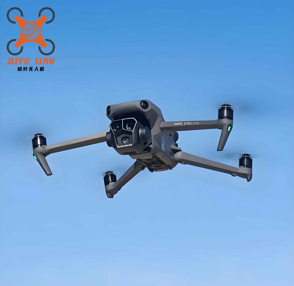
The HMJ-00D4000P quadcopter UAV is selected for this experiment. Its core parameters are shown in the table below.
| Parameter | Value |
|---|---|
| Wheelbase (mm) | 920 |
| Takeoff Weight (kg) | 9.5 |
| Flight Speed (m/s) | 10 |
| Relative Flight Altitude (m) | 1000 |
| Flight Endurance (min) | 35 |
The data communication module is the core device for achieving multi-machine collaborative communication between the ground control center and the quadcopter UAV formation. It mainly includes three types of communication paths: formation wireless data transmission networking module, formation coordination, and remote control emergency communication link, providing support for formation multi-machine state synchronization, command issuance, and emergency intervention.
In experimental debugging and emergency scenarios, the remote control system is necessary to achieve manual control operations such as overall formation emergency stop, single-machine attitude fine-tuning, and formation switching, ensuring flight safety and equipment protection during the experimental phase. The FlySky FS-i6S remote controller and FS-R6B receiver are used to build the formation emergency remote control system.
The FS-i6S remote controller operates in the 2.4 GHz frequency band, supports 10-channel signal output, is equipped with an enhanced external gain antenna, and is compatible with SBUS/PPM dual protocols with the receiver. After frequency pairing, the signal transmission distance can reach 1.5 km, with strong anti-multi-machine interference capability, meeting the needs for synchronous control input, formation mode switching, and emergency command issuance for formations of up to 10 UAVs. The FS-R6B receiver has an input voltage range of 5 to 7.4 V, uses a miniaturized surface-mount design suitable for UAV body installation space, and is equipped with 6 independent PWM channels and 1 bidirectional SBUS channel. It supports both independent control signal reception for a single UAV and unified command distribution for the formation through the SBUS channel, simplifying wiring complexity with the formation main control module.
Communication between the ground receiving station and the main controller of each UAV in the formation is established through LoRa wireless data transmission networking, forming a 1-to-16 star network topology. This meets the parallel transmission requirements of multi-UAV formation data. Through the networking module, each UAV can upload its real-time status information to the ground control station, and can receive formation reference trajectories, formation adjustment commands, and parameter tuning signals from the formation, providing experimental data support for formation communication delay detection.
Control Metrics
Five UAVs are selected, numbered #1 to #5. The formation attitude consistency error is used to validate formation steady-state accuracy, defined as the maximum deviation between the heading angles of all wingman UAVs and the heading angle of the leader UAV. This metric reflects the degree of attitude synchronization among UAVs in the formation; the smaller the error, the more precise the formation attitude coordination.
In our experiments, all UAVs’ attitude errors rapidly rise from about -4 degrees to approximately 4 degrees. However, the error curves for each UAV exhibit identical fluctuation trends. The individual error differences are close to zero, indicating that the attitude-coupled input allows the formation to achieve attitude synchronization from the start-up phase. This demonstrates the effectiveness of the attitude-coupled input design in ensuring the precision of formation attitude coordination.
Three-dimensional UAV formation configuration control intrinsically tests the multi-dimensional coordination ability and anti-interference capability of the formation control method. In three-dimensional space, each UAV should be able to maintain the preset formation distribution, and during trajectory tracking, attitude and position adjustments should be smooth, avoiding overshoot or oscillation. In our results, at the same X position, the Y coordinates of all UAVs are concentrated in the 3 to 5 m interval, and the Z coordinates are concentrated in the 6 to 10 m interval. This indicates that the formation can maintain the preset distribution in three-dimensional space, rather than having individual UAVs detach from the cluster, demonstrating three-dimensional position coordination. Furthermore, all trajectories along the X direction from 0 to 25 m are continuous without drastic fluctuations, corresponding to smooth dynamic response and ensuring that during configuration switching or trajectory tracking, attitude and position adjustments are smooth, avoiding overshoot or oscillation.
Control Effect Analysis
We compare the formation attitude consistency errors using five methods: distributed adaptive event-triggered formation control, high-order sliding mode differentiator-based formation control, RBF and BP neural network-based formation control, fixed-time disturbance observer-based formation control, and our joint variable universe fuzzy PID control method.
| Method | Attitude Consistency Error Characteristics |
|---|---|
| Distributed Adaptive Event Triggered | Evident discrete characteristics; approximately 2.6° error in initial phase; inter-UAV error differences around 1.5°; sustained error dispersion leads to accumulated tracking errors. |
| High-Order Sliding Mode Differentiator | Simultaneous fluctuation and dispersion; error peak near ±4° in initial phase; inter-UAV error difference reaches 3.5°; periodic fluctuations and persistent dispersion cause minor attitude oscillations during landing. |
| RBF and BP Neural Networks | Most prominent issues; maximum error up to 3.8° in initial phase; inter-UAV differences over 2.3°; high dispersion persists, leading to tracking errors exceeding thresholds and cluster detachment. |
| Fixed-Time Disturbance Observer | Consistent notable deviation; error peak around ±3° in initial phase; inter-UAV error difference about 2.2°; high dispersion throughout due to insufficient estimation accuracy for time-varying unstructured disturbances. |
| Joint Variable Universe Fuzzy PID (Ours) | Error curves perfectly consistent in trend; inter-UAV error differences always below 0.5° in initial phase; error magnitude reduces to ±0.1° with differences below 0.1° in steady-state; high-precision attitude synchronization without collision risks. |
Table: Comparison of formation attitude consistency errors for different methods.
The distributed adaptive event-triggered method only adjusts the trigger threshold adaptively, without considering the need for increased sampling frequency during UAV attitude switching, leading to lagged control command updates and accumulated tracking errors, eventually causing single UAV detachment. The high-order sliding mode differentiator, while reducing chattering, still exhibits high-frequency minor perturbations causing micro-fluctuations in UAV attitude adjustments, reducing position synchronization during landing and increasing collision risk. The RBF and BP neural network methods suffer from time lag in weight adjustment under complex conditions, leading to trajectory deviations beyond limits and detachment. The fixed-time disturbance observer has limited estimation accuracy for landing-phase time-varying disturbances, and does not dynamically correct individual initial deviations or actuator errors, ultimately causing detachment. Our method, by dynamically adjusting the fuzzy rule universe based on real-time tracking errors and combining it with PID for steady-state accuracy, excels in adapting to time-varying disturbances and attitude changes, effectively suppressing individual position deviations and preventing UAV detachment.
We further validate the robustness and adaptability of the control strategy under three wind speed conditions (breeze, strong wind) and three obstacle density scenarios (low, medium, high). The same experimental equipment is used for all five formation control methods. Evaluation metrics include trajectory tracking error variance, obstacle avoidance success rate, and energy consumption efficiency.
| Wind | Obstacle | Method | Tracking Error Variance (m²) | Avoidance Success Rate (%) | Energy Efficiency (%) |
|---|---|---|---|---|---|
| Breeze | Low | Distributed Adaptive Event Triggered | 0.12 | 95 | 88 |
| High-Order Sliding Mode | 0.15 | 93 | 86 | ||
| RBF and BP Neural Networks | 0.18 | 90 | 84 | ||
| Fixed-Time Disturbance Observer | 0.14 | 94 | 87 | ||
| Medium | Distributed Adaptive Event Triggered | 0.25 | 90 | 85 | |
| High-Order Sliding Mode | 0.28 | 88 | 83 | ||
| RBF and BP Neural Networks | 0.32 | 85 | 81 | ||
| Fixed-Time Disturbance Observer | 0.27 | 89 | 84 | ||
| High | Distributed Adaptive Event Triggered | 0.40 | 85 | 82 | |
| High-Order Sliding Mode | 0.43 | 83 | 80 | ||
| RBF and BP Neural Networks | 0.48 | 80 | 78 | ||
| Fixed-Time Disturbance Observer | 0.42 | 84 | 81 | ||
| Breeze | Low | Joint Variable Universe Fuzzy PID (Ours) | 0.08 | 98 | 90 |
| Medium | Joint Variable Universe Fuzzy PID (Ours) | 0.18 | 95 | 87 | |
| High | Joint Variable Universe Fuzzy PID (Ours) | 0.30 | 90 | 84 | |
| Strong Wind | Low | Distributed Adaptive Event Triggered | 0.35 | 88 | 80 |
| High-Order Sliding Mode | 0.38 | 86 | 78 | ||
| RBF and BP Neural Networks | 0.42 | 83 | 76 | ||
| Fixed-Time Disturbance Observer | 0.37 | 87 | 79 | ||
| Medium | Distributed Adaptive Event Triggered | 0.55 | 80 | 75 | |
| High-Order Sliding Mode | 0.58 | 78 | 73 | ||
| RBF and BP Neural Networks | 0.63 | 75 | 71 | ||
| Fixed-Time Disturbance Observer | 0.57 | 79 | 74 | ||
| High | Distributed Adaptive Event Triggered | 0.75 | 70 | 70 | |
| High-Order Sliding Mode | 0.78 | 68 | 68 | ||
| RBF and BP Neural Networks | 0.83 | 65 | 66 | ||
| Fixed-Time Disturbance Observer | 0.77 | 69 | 69 | ||
| Strong Wind | Low | Joint Variable Universe Fuzzy PID (Ours) | 0.25 | 92 | 82 |
| Medium | Joint Variable Universe Fuzzy PID (Ours) | 0.45 | 85 | 77 | |
| High | Joint Variable Universe Fuzzy PID (Ours) | 0.65 | 75 | 72 |
Table: Performance comparison of different methods under various wind and obstacle conditions.
From the table, under all tested wind and obstacle conditions, the joint variable universe fuzzy PID method consistently achieves the best performance across all evaluation metrics. Our method’s trajectory tracking error variance is as low as 0.08 m² under low obstacle density in a breeze and 0.65 m² under high obstacle density in strong wind, both lower than those of other methods. The obstacle avoidance success rate reaches as high as 98% under low obstacle density in a breeze and 75% under high obstacle density in strong wind, maintaining a high level. The energy consumption efficiency is also superior, at 90% under low obstacle density in a breeze and 72% under high obstacle density in strong wind. In contrast, other methods show increasing trajectory tracking error variance, decreasing obstacle avoidance success rates, and declining energy consumption efficiency as wind strength and obstacle density increase. This strongly validates that our joint variable universe fuzzy PID control strategy possesses superior robustness and adaptability.
Conclusion
In our work on China drone formation control, we have successfully proposed and implemented a joint variable universe fuzzy PID control method coupled with wingman attitude to address the core issues of low attitude coordination accuracy and difficulty in maintaining formation configuration for quadcopter UAV formations in complex dynamic environments. By designing a real-time relative state input mechanism based on heading angle fusion, we effectively solved the orientation misjudgment and control lag inherent in traditional global coordinate systems. The introduction of collaborative scaling factors for adaptive universe adjustment significantly enhanced the system’s dynamic adaptability to nonlinear disturbances and multi-UAV coupling. Combined with an independent parameter collaborative tuning strategy, we suppressed integral saturation and noise amplification while improving overall formation robustness and single-machine correction performance. Experimental results show that our method maintains attitude consistency error individual differences below 0.5° and achieves stable centralized 3D configuration even under strong interference scenarios. This not only validates the effectiveness and advancements of our control strategy but also provides a highly reliable and high-precision formation control solution for practical applications such as low-altitude logistics and dense collaborative operations, demonstrating clear engineering application value and theoretical significance for the advancement of China drone swarm technology.