
In modern warfare, the coordinated operation of multiple unmanned aerial vehicles (UAVs) has become increasingly prevalent for executing various combat missions, particularly evident in several high-tech localized conflicts, drawing global attention. As a key technology within multi-UAV cooperation, drone formation coordination has spurred extensive research among scholars worldwide. Currently, multi-drone formation coordination primarily employs centralized and distributed approaches. Centralized formation control methods rely on a central computational node, offering high control effectiveness and precision but demanding robust communication and computing capabilities. In contrast, distributed formation control methods operate without a central node; although they may yield lower control accuracy compared to centralized systems, they exhibit superior robustness and adaptability, along with enhanced survivability in battlefield environments. In this paper, I focus on distributed multi-drone formation coordination based on consensus theory.
Consensus refers to the process where each agent interacts with others according to specific rules, ultimately leading to the convergence of certain states across all agents. Building upon consensus theory, multi-drone formation coordination has achieved notable progress. However, most existing studies consider communication delays arising from inter-drone interactions, while relatively fewer address input delays resulting from onboard information processing. Input delays can significantly impact system stability and performance, making their analysis crucial for practical implementations. Therefore, in this work, I investigate distributed drone formation coordination in three-dimensional space, accounting for heterogeneous time-varying input delays. I employ a second-order consensus protocol to address the formation problem and analyze the effects of these delays on system stability. By constructing and analyzing Lyapunov-Krasovskii functionals, I derive sufficient conditions for consensus under directed communication topologies. The maximum allowable input delays can be determined by solving linear matrix inequalities (LMIs). Simulation experiments validate the effectiveness of the proposed approach and conclusions.
The coordination of drone formations is essential for tasks such as surveillance, reconnaissance, and collaborative attacks. Distributed control strategies offer scalability and fault tolerance, which are critical in dynamic and adversarial environments. However, the presence of delays—whether from communication or internal processing—can degrade performance or even lead to instability. Thus, understanding and mitigating these effects is vital. In this paper, I delve into the mathematical modeling and stability analysis of drone formations with input delays, providing a framework that can be extended to real-world applications.
To set the stage, let me define the multi-drone system. Consider a group of n drones operating in three-dimensional space. The communication topology among drones is represented by a directed graph G = (V, E, A), where V = {v1, v2, …, vn} denotes the set of drone nodes, E is the edge set, and A = [aij] is the adjacency matrix. An edge eij = (vi, vj) ∈ E indicates that drone j can transmit its position and velocity information to drone i. The neighbor set of drone i is denoted by Ni. The Laplacian matrix L = [lij] is defined as lii = Σj≠i aij and lij = -aij for i ≠ j. A directed graph is said to be connected if it contains a globally reachable node, meaning there exists a node from which all other nodes are reachable via directed paths.
The nonlinear dynamics of each drone are modeled based on standard aerodynamic principles. For drone i, the equations of motion in three-dimensional inertial coordinates are given by:
$$ \begin{aligned}
\dot{x}_i &= V_i \cos \chi_i \cos \phi_i, \\
\dot{y}_i &= V_i \cos \chi_i \sin \phi_i, \\
\dot{z}_i &= V_i \sin \chi_i, \\
\dot{V}_i &= a_{i1} – g \sin \chi_i, \\
\dot{\chi}_i &= \frac{1}{V_i} (a_{i2} \cos \chi_i – g \cos \chi_i), \\
\dot{\phi}_i &= \frac{a_{i3}}{V_i \cos \chi_i},
\end{aligned} $$
where (x_i, y_i, z_i) represents the inertial position, V_i is the speed, χ_i is the pitch angle, φ_i is the heading angle, and (a_{i1}, a_{i2}, a_{i3}) are control inputs corresponding to tangential and normal accelerations. For formation control purposes, I linearize this model and define a new control input u_i = [u_{xi}, u_{yi}, u_{zi}]^T, representing accelerations along the inertial coordinate axes. The transformed dynamics can be expressed as a second-order system:
$$ \begin{aligned}
\dot{\boldsymbol{\xi}}_i &= \boldsymbol{\varsigma}_i, \\
\dot{\boldsymbol{\varsigma}}_i &= \boldsymbol{u}_i,
\end{aligned} $$
where ξ_i = [x_i, y_i, z_i]^T and ς_i = [ẋ_i, ẏ_i, ż_i]^T. This simplified model captures the essential kinematics for formation control, facilitating the application of consensus protocols.
In drone formation coordination, the objective is to achieve and maintain a desired geometric pattern while following a common reference velocity. Let r_i denote the relative position vector of drone i with respect to the formation center, and let ς* be the reference velocity. The formation error for drone i is defined as ξ_i – r_i and ς_i – ς*. A consensus-based protocol aims to drive these errors to zero or to a small neighborhood, ensuring cohesive movement.
To account for input delays, which arise from onboard computation and actuation lags, I introduce time-varying delays τ_i(t) for each drone, satisfying 0 ≤ τ_i(t) ≤ h_i, where h_i > 0 is the delay upper bound. These delays are heterogeneous, meaning they can vary across drones. The second-order consensus protocol with input delays is formulated as:
$$ \begin{aligned}
\boldsymbol{u}_i(t) &= -k_1 \sum_{j \in N_i} [\boldsymbol{\varsigma}_i(t – \tau_i(t)) – \boldsymbol{\varsigma}_j(t – \tau_i(t))] \\
&\quad – k_2 \sum_{j \in N_i} [(\boldsymbol{\xi}_i(t – \tau_i(t)) – \boldsymbol{r}_i) – (\boldsymbol{\xi}_j(t – \tau_i(t)) – \boldsymbol{r}_j)] \\
&\quad – k_3 [\boldsymbol{\varsigma}_i(t – \tau_i(t)) – \boldsymbol{\varsigma}^*],
\end{aligned} $$
where k_1, k_2, k_3 > 0 are control gains. This protocol integrates relative velocity and position feedback with a reference velocity term, adjusted for delays. The goal is to achieve ς_i(t) → ς* and ξ_i(t) – r_i → ξ_j(t) – r_j for all i, j, implying formation convergence.
To analyze stability, I define error variables ẑ_i(t) = ς_i(t) – ς* and ẋ_i(t) = ξ_i(t) – r_i – ξ*(t), where ξ*(t) is a reference trajectory. However, for simplicity, I assume the formation center moves with constant velocity ς*, so ξ*(t) = ς* t. The collective dynamics can be written in vector form. Let y(t) = [ξ(t)^T, ς(t)^T]^T, where ξ = [ξ_1^T, …, ξ_n^T]^T and ς = [ς_1^T, …, ς_n^T]^T. The system becomes:
$$ \dot{\boldsymbol{y}}(t) = \boldsymbol{A} \boldsymbol{y}(t) + \sum_{i=1}^n \boldsymbol{B}_i \boldsymbol{y}(t – \tau_i(t)), $$
with appropriate matrices A and B_i derived from the protocol and graph Laplacian. This representation allows for stability analysis using Lyapunov-Krasovskii methods.
The stability of the drone formation under input delays hinges on the properties of the communication graph and the delay bounds. For directed graphs containing a globally reachable node, I establish sufficient conditions for consensus. The key tool is the construction of a Lyapunov-Krasovskii functional that incorporates integral terms to account for delays. By applying Jensen’s inequality and other matrix techniques, I derive LMIs that guarantee asymptotic stability.
Specifically, consider the functional candidate:
$$ V(t) = \boldsymbol{y}(t)^T \boldsymbol{P} \boldsymbol{y}(t) + \sum_{i=1}^n \int_{t-h_i}^t \dot{\boldsymbol{y}}(s)^T \boldsymbol{R}_i \dot{\boldsymbol{y}}(s) \, ds, $$
where P > 0 and R_i > 0 are symmetric positive definite matrices. The time derivative of V(t) along trajectories yields terms involving delays. Using bounding inequalities, I obtain:
$$ \dot{V}(t) \leq \boldsymbol{\eta}(t)^T \boldsymbol{\Psi} \boldsymbol{\eta}(t), $$
where η(t) is an augmented state vector including delayed states, and Ψ is a matrix dependent on system parameters and delays. The condition Ψ < 0 ensures negativity of Ȯ(t), implying consensus.
The main result is summarized in the following theorem, which provides a computable criterion for stability.
Theorem 1. For a directed communication graph that is connected (i.e., contains a globally reachable node), the drone formation system with heterogeneous input delays achieves consensus if there exist matrices P > 0, R_i > 0, and scalars h_i > 0 such that the following linear matrix inequality holds:
$$ \begin{bmatrix}
\boldsymbol{\Psi}_{11} & \boldsymbol{\Psi}_{12} & \boldsymbol{\Psi}_{13} \\
* & \boldsymbol{\Psi}_{22} & \boldsymbol{\Psi}_{23} \\
* & * & \boldsymbol{\Psi}_{33}
\end{bmatrix} < 0, $$
where the blocks are defined as:
$$ \begin{aligned}
\boldsymbol{\Psi}_{11} &= \boldsymbol{P} \boldsymbol{A} + \boldsymbol{A}^T \boldsymbol{P} – \sum_{i=1}^n h_i^{-1} \boldsymbol{R}_i + \sum_{i=1}^n h_i \boldsymbol{A}^T \boldsymbol{R}_i \boldsymbol{A}, \\
\boldsymbol{\Psi}_{12} &= [\boldsymbol{P} \boldsymbol{B}_1 + h_1^{-1} \boldsymbol{R}_1, \ldots, \boldsymbol{P} \boldsymbol{B}_n + h_n^{-1} \boldsymbol{R}_n], \\
\boldsymbol{\Psi}_{13} &= [h_1 \boldsymbol{A}^T \boldsymbol{R}_1 \boldsymbol{B}_1, \ldots, h_n \boldsymbol{A}^T \boldsymbol{R}_n \boldsymbol{B}_n], \\
\boldsymbol{\Psi}_{22} &= \text{diag}(-h_1^{-1} \boldsymbol{R}_1, \ldots, -h_n^{-1} \boldsymbol{R}_n), \\
\boldsymbol{\Psi}_{23} &= \text{block-diag}(h_1 \boldsymbol{B}_1^T \boldsymbol{R}_1 \boldsymbol{B}_1, \ldots, h_n \boldsymbol{B}_n^T \boldsymbol{R}_n \boldsymbol{B}_n), \\
\boldsymbol{\Psi}_{33} &= \text{diag}(-h_1 \boldsymbol{R}_1, \ldots, -h_n \boldsymbol{R}_n).
\end{aligned} $$
Here, * denotes symmetric entries. The maximum allowable delays h_i can be found by solving this LMI using numerical tools like MATLAB’s LMI toolbox. This theorem extends existing results by accommodating heterogeneous delays and directed topologies, which are common in practical drone formations.
To illustrate the application of this theorem, I present a simulation case study involving five drones. The communication topology is described by the Laplacian matrix:
$$ \boldsymbol{L} = \begin{bmatrix}
1 & -1 & 0 & 0 & 0 \\
0 & 0 & 0 & 0 & 0 \\
0 & -1 & 1 & 0 & 0 \\
0 & -1 & 0 & 1 & 0 \\
0 & -1 & 0 & 0 & 1
\end{bmatrix}. $$
This directed graph has a globally reachable node (e.g., node 1), ensuring information propagation. The control gains are set to k_1 = 0.8, k_2 = 1, k_3 = 1. Solving the LMI yields maximum delay bounds: h_1 = 0.157, h_2 = 0.171, h_3 = 0.183, h_4 = 0.210, h_5 = 0.224 seconds. I then assign time-varying delays within these bounds:
$$ \begin{aligned}
\tau_1(t) &= 0.15 |\sin(10t)|, \\
\tau_2(t) &= 0.17 |\cos(10t)|, \\
\tau_3(t) &= 0.18 |\sin(10t)|, \\
\tau_4(t) &= 0.21 |\cos(10t)|, \\
\tau_5(t) &= 0.22 |\sin(10t)|.
\end{aligned} $$
The initial conditions for the drones are provided in the table below, including positions, velocities, and orientation angles.
| Drone ID | Initial Position (m) | Initial Velocity (m/s) | Initial Pitch Angle (rad) | Initial Heading Angle (rad) |
|---|---|---|---|---|
| 1 | (100, 154, 180) | 17 | 0 | 0 |
| 2 | (200, 160, 120) | 20 | -0.2 | 0.3 |
| 3 | (140, 200, 250) | 25 | 0.4 | -0.1 |
| 4 | (170, 320, 120) | 28 | -0.6 | 0.3 |
| 5 | (290, 250, 300) | 33 | 0.1 | -0.7 |
The desired formation is defined by relative offset vectors: r_1 = (0, 0, 0), r_2 = (100, 0, 0), r_3 = (0, 100, 0), r_4 = (0, 0, 100), r_5 = (100, 100, 100) meters, and the reference velocity is ς* = [25, 20, 2]^T m/s. This configuration corresponds to a rectangular prism pattern moving at a constant velocity. To quantify formation accuracy, I define an error function:
$$ E(t) = \frac{1}{2} \sum_{i=1}^n \sum_{j \in N_i} \left\| (\boldsymbol{\xi}_i – \boldsymbol{r}_i) – (\boldsymbol{\xi}_j – \boldsymbol{r}_j) \right\|^2, $$
which measures the sum of squared position deviations from the desired geometry. Convergence of E(t) to zero indicates successful formation attainment.
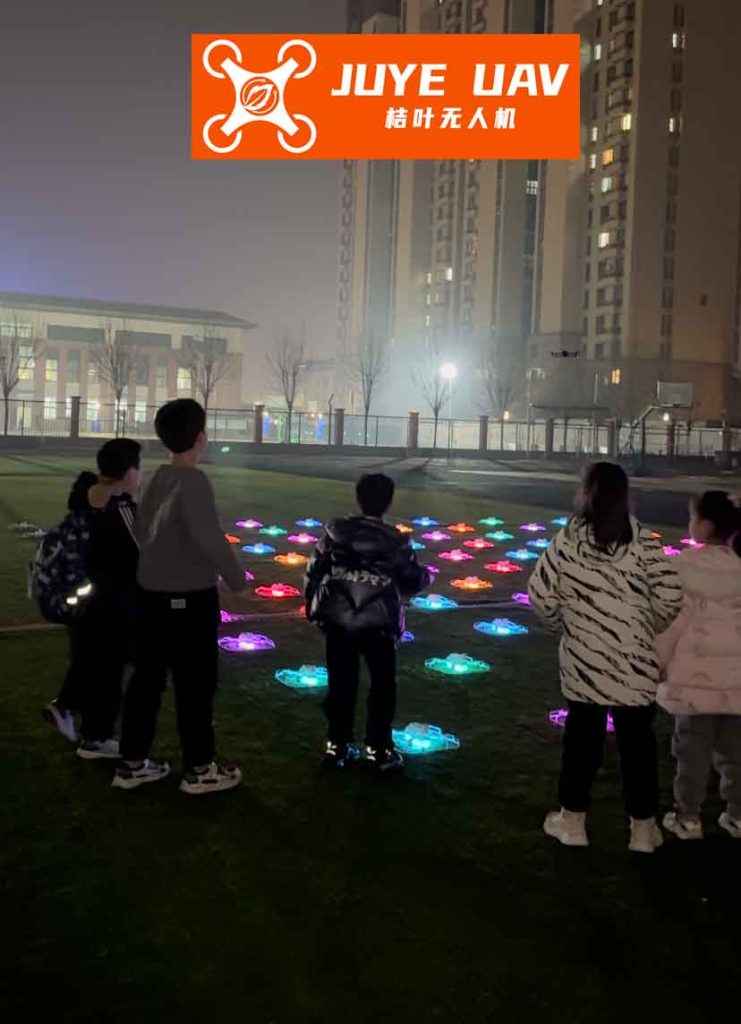
The simulation results demonstrate the effectiveness of the proposed protocol. Over time, the drones align their velocities to the reference and arrange themselves into the specified formation, despite the presence of input delays. The following figure illustrates a snapshot of a drone formation in action, highlighting the coordinated patterns achievable with distributed control.
In the simulation, the position trajectories along the x-axis converge to coordinated values, maintaining the relative offsets. The velocity profiles show all drones approaching the reference velocity ς* within a few seconds. The error function E(t) decays to near zero, confirming formation stability. These outcomes validate the theoretical predictions and underscore the robustness of the consensus-based approach to input delays.
To further analyze performance, I examine the sensitivity of the system to delay variations. When delays exceed the computed bounds, oscillations or divergence may occur, emphasizing the importance of accurate delay estimation and compensation. In practice, adaptive techniques could be incorporated to handle uncertain or time-varying delays, enhancing the resilience of drone formations in dynamic environments.
The drone formation coordination problem is inherently multi-disciplinary, involving control theory, graph theory, and network systems. The consensus protocol employed here leverages local information exchange, reducing communication overhead and promoting scalability. However, challenges remain, such as dealing with packet loss, bandwidth limitations, and nonlinear dynamics. Future work could integrate robust control methods, such as H-infinity or sliding mode control, to address these issues while maintaining formation integrity.
Moreover, the application of drone formations extends beyond military domains to civilian uses like light shows, agricultural monitoring, and disaster response. For instance, synchronized drone light shows rely on precise formation control to create intricate aerial displays. The principles discussed in this paper can be adapted to such scenarios, where timing and coordination are paramount. The image above depicts a formation drone light show, illustrating the artistic potential of coordinated UAVs.
In conclusion, distributed drone formation coordination offers a viable solution for multi-UAV systems, particularly in environments where centralized control is impractical. Input delays, arising from onboard processing, can significantly impact stability, but through careful analysis using Lyapunov-Krasovskii functionals and LMI techniques, sufficient conditions for consensus can be established. The proposed method accommodates heterogeneous time-varying delays and directed communication topologies, making it applicable to real-world settings. Simulation results confirm that drones can achieve and maintain desired formations under delay constraints, with error convergence validating the approach.
This work contributes to the broader field of multi-agent systems by providing a framework for delay-tolerant formation control. Future directions include extending the analysis to higher-order dynamics, incorporating obstacle avoidance, and testing in hardware experiments. As drone technology advances, robust formation algorithms will play a crucial role in enabling complex collaborative tasks, from autonomous swarms to intelligent transportation systems. The key takeaway is that with proper design, distributed drone formations can withstand practical imperfections like delays, ensuring reliable and scalable operations.
Throughout this paper, I have emphasized the importance of drone formation coordination, repeatedly highlighting how consensus-based strategies can address challenges posed by input delays. By integrating theoretical rigor with simulation validation, I have demonstrated a pathway toward resilient and adaptive multi-drone systems. The continued evolution of this field promises to unlock new capabilities for UAV applications, driven by innovations in control theory and networked systems.