
The spectacle of a coordinated formation drone light show is a mesmerizing demonstration of modern technology, where hundreds of unmanned aerial vehicles (UAVs) move in perfect harmony to create intricate, luminous patterns in the night sky. Beyond their entertainment value, these systems represent the pinnacle of multi-agent coordination, with applications ranging from search and rescue to precision agriculture and automated logistics. The fundamental challenge enabling such a breathtaking formation drone light show lies in the design of robust control algorithms that ensure each drone maintains its precise position relative to its neighbors, despite real-world imperfections. Chief among these imperfections is communication delay.
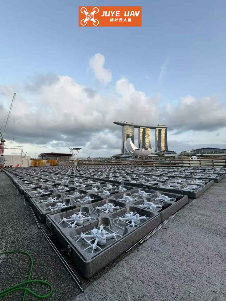
In any multi-drone system aiming to achieve a stable formation, such as that required for a flawless formation drone light show, individual agents must constantly exchange state information like position and velocity. This communication almost invariably occurs over a shared network, be it radio or a dedicated control link. Due to inherent limitations like finite bandwidth, data packet congestion, or external electromagnetic interference, the transmission of this vital information is often subject to time-varying delays. These delays are not merely constant lags; they are frequently random and unpredictable. If unaccounted for, such delays can introduce oscillations, instability, or even cause the entire formation to break apart—a catastrophic failure for any aerial performance. Therefore, the development of control strategies that explicitly account for and compensate for these stochastic communication delays is paramount for realizing reliable and scalable systems, especially for large-scale, complex formation drone light show displays. This article delves into the design of a decentralized formation control protocol for vertical take-off and landing (VTOL) UAVs, explicitly modeling the randomness of communication delays and providing a rigorous stability guarantee, thereby paving the way for more robust and delay-tolerant autonomous swarms.
System Modeling and Problem Formulation
We consider a group of \(n\) VTOL UAVs, indexed by \(i \in \mathcal{N} := \{1, 2, …, n\}\). The objective is for these agents to achieve and maintain a desired geometric formation defined by constant offsets \(\delta_{ij} \in \mathbb{R}^3\), while also stabilizing their linear velocities to zero (a hovering state). The communication topology among the drones is modeled as an undirected, connected graph \(\mathcal{G} = (\mathcal{N}, \mathcal{E}, K)\), where \(\mathcal{E}\) is the set of communication links and \(K = [k_{ij}] \in \mathbb{R}^{n \times n}\) is the symmetric weighted adjacency matrix with \(k_{ij} > 0\) if \((i, j) \in \mathcal{E}\) and \(k_{ii}=0\).
1.1 VTOL UAV Nonlinear Dynamics
The dynamics of each VTOL UAV are separated into translational (position) and rotational (attitude) subsystems, which are coupled through the thrust direction.
Translational Dynamics:
$$ \begin{cases}
\dot{p}_i = v_i \\
\dot{v}_i = g e_3 – \frac{\Lambda_i}{m_i} R(Q_i)^T e_3
\end{cases} $$
Here, \(p_i, v_i \in \mathbb{R}^3\) are the position and linear velocity of the \(i\)-th drone in an inertial frame. \(m_i\) is its mass, \(g\) is gravitational acceleration, and \(e_3 = (0,0,1)^T\). \(\Lambda_i \in \mathbb{R}\) is the magnitude of the total thrust force. \(Q_i = (q_i^T, \eta_i)^T \in \mathbb{R}^4\) is the unit quaternion representing the drone’s attitude, and \(R(Q_i) \in SO(3)\) is the corresponding rotation matrix mapping body-frame vectors to the inertial frame.
Rotational Dynamics:
$$ \begin{cases}
\dot{Q}_i = \frac{1}{2} T(Q_i) \omega_i \\
J_i \dot{\omega}_i = \Gamma_i – S(\omega_i) J_i \omega_i
\end{cases} $$
Here, \(\omega_i \in \mathbb{R}^3\) is the angular velocity in the body frame, \(J_i = J_i^T > 0\) is the inertia matrix, and \(\Gamma_i \in \mathbb{R}^3\) is the control torque input. The matrices \(T(Q_i)\) and \(S(\cdot)\) are standard for quaternion and cross-product operations.
1.2 Random Communication Delay Model
The core challenge we address is that the information exchange between neighboring drones, crucial for calculating relative positions, is subject to random delays. We model this phenomenon using a Bernoulli distributed random variable. Let \(\tau_{ij}(t) \leq \tau\) be a time-varying delay in the communication from drone \(j\) to drone \(i\). We introduce a stochastic variable \(\lambda(t)\):
$$
\text{Prob}\{\lambda(t) = 1\} = \mathbb{E}\{\lambda\} = \bar{\lambda}, \quad \text{Prob}\{\lambda(t) = 0\} = 1 – \bar{\lambda}
$$
where \(\bar{\lambda} \in [0, 1]\). The interpretation is:
- When \(\lambda(t)=1\), the communication is instantaneous (or delay-free for control purposes).
- When \(\lambda(t)=0\), the information from neighbors is received with a delay \(\tau_{ij}(t)\).
This model effectively captures the sporadic and random nature of network-induced delays, a more realistic scenario for a formation drone light show operating in a potentially congested wireless environment than assuming a constant delay.
Controller Design
The control design follows a hierarchical strategy. First, an intermediate control force \(F_i \in \mathbb{R}^3\) is designed based on delayed neighbor information to achieve formation-keeping in the translational dynamics. From \(F_i\), the required thrust magnitude \(\Lambda_i\) and a desired attitude \(Q_{di}\) are extracted. Second, a torque controller \(\Gamma_i\) is designed to make the actual attitude \(Q_i\) track \(Q_{di}\). This decoupling simplifies the design and analysis.
2.1 Translational Subsystem Control
We define formation tracking errors. Let \(\xi_i = p_i – \theta_i – \alpha_i\) and \(z_i = \dot{\xi}_i\), where \(\theta_i\) and \(\alpha_i\) are auxiliary filter states. The intermediate control force \(F_i\) and the filter dynamics are designed as follows:
$$
\begin{aligned}
F_i &= -k_i^p \chi(\theta_i) – k_i^d \chi(\dot{\theta}_i) \\
\ddot{\theta}_i &= F_i – u_i \\
\ddot{\alpha}_i &= u_i – \varphi_i – \frac{\Lambda_i}{m_i} \Pi_i \tilde{q}_i
\end{aligned}
$$
where \(k_i^p, k_i^d > 0\) are gains, \(\chi(\cdot)\) is a smooth saturation function (to ensure \(F_i\) remains within feasible bounds), and \(u_i = -L_i^p \alpha_i – L_i^d \dot{\alpha}_i\) is a stabilizing term for the \(\alpha_i\) dynamics. The term \(\Pi_i \tilde{q}_i\) represents the attitude misalignment effect, with \(\tilde{q}_i\) being the vector part of the attitude error quaternion \(\tilde{Q}_i = Q_{di}^{-1} \otimes Q_i\).
The critical term \(\varphi_i\) incorporates the formation feedback with random delays:
$$
\varphi_i = -k_i^v z_i – \sum_{j=1}^{n} k_{ij} \left[ \lambda \xi_{ij}(t) + (1-\lambda) \xi_{ij}(t-\tau_{ij}(t)) \right]
$$
where \(k_i^v > 0\) is a gain, and \(\xi_{ij} = \xi_i – \xi_j – \delta_{ij}\) is the relative formation error. When \(\lambda=1\), the current error \(\xi_{ij}(t)\) is used. When \(\lambda=0\), the delayed error \(\xi_{ij}(t-\tau_{ij})\) is used. This controller uses the available (potentially outdated) information to compute corrective actions, making it suitable for a formation drone light show network.
Once \(F_i\) is computed, the actual thrust magnitude and desired attitude are extracted via:
$$
\Lambda_i = m_i \|g e_3 – F_i\|, \quad Q_{di} = \text{Extraction}(F_i)
$$
The extraction algorithm solves for the attitude \(Q_{di}\) whose thrust direction, when multiplied by \(\Lambda_i\), produces the vector \(m_i g e_3 – F_i\).
2.2 Rotational Subsystem Control
The goal is to drive the actual attitude \(Q_i\) to the desired \(Q_{di}\). Defining the attitude error \(\tilde{Q}_i = Q_{di}^{-1} \otimes Q_i = (\tilde{q}_i^T, \tilde{\eta}_i)^T\) and the angular velocity error \(\tilde{\omega}_i = \omega_i – R(\tilde{Q}_i)^T \omega_{di}\) (where \(\omega_{di}\) is derived from \(F_i\)), we design the control torque as:
$$
\Gamma_i = H_i(\cdot) + J_i \dot{\beta}_i – k_i^q \tilde{q}_i – k_i^{\Omega} (\tilde{\omega}_i – \beta_i)
$$
with \(\beta_i = -k_i^{\beta} \tilde{q}_i\). The term \(H_i(\cdot) = S(\omega_i)J_i\omega_i – J_i S(\tilde{\omega}_i)R(\tilde{Q}_i)\omega_{di} + J_i R(\tilde{Q}_i)\dot{\omega}_{di}\) compensates for nonlinear dynamics and feedforward terms. The gains \(k_i^q, k_i^{\Omega}, k_i^{\beta} > 0\) provide proportional and derivative feedback on the attitude error.
Stability Analysis
The stability of the closed-loop system is analyzed using stochastic Lyapunov theory. We construct a composite Lyapunov-Krasovskii functional candidate that accounts for the current states and the delayed error information.
Theorem 1 (Formation under Random Delays). Consider the multi-UAV system (1)-(2) under the control laws (3)-(6). Assume the communication graph \(\mathcal{G}\) is undirected and connected. If the control gains \(k_i^p, k_i^d, k_i^v\) are chosen such that:
1. \(\sqrt{3}\sigma_b (k_i^p + k_i^d) < g\) (to ensure feasible thrust extraction),
2. \(k_i^z := k_i^v – \frac{1}{2}\sum_{j=1}^n k_{ij} \left[ (\bar{\lambda}-1)\epsilon + \frac{\tau^2}{\epsilon} \right] > 0\) for some \(\epsilon > 0\),
where \(\sigma_b\) is the bound of the saturation function \(\chi(\cdot)\), then for any initial conditions and any random delay sequence satisfying \(\tau_{ij}(t) \leq \tau\), the following holds almost surely:
- All signals in the closed-loop system remain bounded.
- The formation is achieved asymptotically: \(\lim_{t \to \infty} (p_i(t) – p_j(t)) = \delta_{ij}\).
- The drones stabilize to hover: \(\lim_{t \to \infty} v_i(t) = 0\).
- The attitude tracks the desired one: \(\lim_{t \to \infty} \tilde{q}_i(t) = 0, \lim_{t \to \infty} \tilde{\omega}_i(t) = 0\).
Proof Sketch: The proof proceeds in two main steps, leveraging the separation between rotational and translational error dynamics.
Step 1: Attitude Subsystem Stability. Consider the Lyapunov function candidate for the rotational dynamics:
$$ V_a = \sum_{i=1}^n \left( \frac{1}{2} \Omega_i^T J_i \Omega_i + k_i^q \tilde{q}_i^T \tilde{q}_i + k_i^q (1-\tilde{\eta}_i)^2 \right) $$
where \(\Omega_i = \tilde{\omega}_i – \beta_i\). Using the properties of quaternions \((\tilde{q}_i^T\tilde{q}_i + (1-\tilde{\eta}_i)^2 = 2(1-\tilde{\eta}_i))\) and the control law (6), its derivative can be shown to satisfy:
$$ \dot{V}_a = \sum_{i=1}^n \left( -k_i^{\Omega} \Omega_i^T \Omega_i – k_i^q k_i^{\beta} \tilde{q}_i^T \tilde{q}_i \right) \leq 0 $$
This proves that \(\Omega_i, \tilde{q}_i \in \mathcal{L}_2 \cap \mathcal{L}_{\infty}\), and \(\dot{\Omega}_i \in \mathcal{L}_{\infty}\). By Barbalat’s lemma, we conclude \(\Omega_i \to 0\) and \(\tilde{q}_i \to 0\), which implies \(\tilde{\omega}_i \to 0\). Thus, the attitude tracking objective is achieved.
Step 2: Translational Subsystem Stability. This is the core part dealing with random delays. Define the translational error Lyapunov-Krasovskii functional:
$$ \begin{aligned}
V_t &= \frac{1}{2}\sum_{i=1}^n \left( z_i^T z_i + \frac{1}{2}\sum_{j=1}^n k_{ij} \xi_{ij}^T \xi_{ij} \right) \\
V_k &= \sum_{i=1}^n \sum_{j=1}^n \frac{k_{ij} \tau}{2\epsilon} \int_{-\tau}^{0} \int_{t+s}^{t} z_j^T(\rho) z_j(\rho) \, d\rho \, ds \\
V &= V_t + V_k
\end{aligned} $$
Taking the time derivative of \(V_t\) and using the dynamics \(\dot{z}_i = \varphi_i\) yields terms containing the delayed errors \(\xi_{ij}(t-\tau_{ij})\). The functional \(V_k\) is introduced specifically to handle these terms. Applying Jensen’s inequality and Young’s inequality allows us to bound the derivative. Taking the expectation \(\mathbb{E}\{\dot{V}\}\) and using the properties of the Bernoulli variable \(\lambda\) leads to:
$$ \mathbb{E}\{\dot{V}\} \leq \sum_{i=1}^n \left( -k_i^z z_i^T z_i \right) + \text{(negative terms)} $$
Given condition (2) that \(k_i^z > 0\), we have \(\mathbb{E}\{\dot{V}\} \leq 0\). This establishes that \(z_i \in \mathcal{L}_2 \cap \mathcal{L}_{\infty}\) in expectation. Further analysis using properties of square-integrable signals and Barbalat’s lemma shows that \(z_i \to 0\) and consequently \(\xi_{ij} \to 0\), meaning the formation error converges to zero. The stability of the filter states \(\theta_i\) and \(\alpha_i\) follows from their input-to-state stable dynamics with vanishing inputs (\(z_i, \tilde{q}_i \to 0\)). Finally, since \(v_i = z_i + \dot{\theta}_i + \dot{\alpha}_i\) and \(p_i – p_j – \delta_{ij} = \xi_{ij} + (\theta_i-\theta_j) + (\alpha_i-\alpha_j)\), the main results of Theorem 1 follow. ∎
Simulation Study: A Dynamic Light Show Pattern
To validate the proposed controller, we simulate a scenario inspired by a formation drone light show. Consider \(n=4\) drones tasked with forming and holding a square in the horizontal plane, a basic building block for more complex patterns. The desired offsets are \(\delta_{12}=(2,0,0)^T\), \(\delta_{23}=(0,2,0)^T\), \(\delta_{34}=(-2,0,0)^T\), \(\delta_{41}=(0,-2,0)^T\). The communication graph is a ring: \(\mathcal{E}=\{(1,2),(2,3),(3,4),(4,1)\}\) with weights \(k_{ij}=0.5\).
We model the random delay as \(\tau_{ij}(t) = 0.25(1 + \sin(0.5t))\) seconds, bounded by \(\tau = 0.5s\). The probability of delay is varied to study its impact: \(\bar{\lambda} = 0\) (always delayed), \(\bar{\lambda}=0.5\) (50% chance of delay), \(\bar{\lambda}=0.8\) (20% chance of delay), and \(\bar{\lambda}=1\) (no delay). The saturation function is chosen as \(\chi(s) = \tanh(s)\). Gains are selected to satisfy Theorem 1.
The performance is evaluated by two key metrics relevant to a formation drone light show: 1) the Formation Convergence Time (time for the max pairwise position error to fall below 0.1m), and 2) the Steady-State RMS Error. The results for 20 Monte Carlo runs per \(\bar{\lambda}\) value are summarized below.
| Delay Probability \((1-\bar{\lambda})\) | Avg. Convergence Time (s) | Avg. Steady-State RMS Error (m) | Max Overshoot (m) |
|---|---|---|---|
| 100% \((\bar{\lambda}=0)\) | 8.7 | 0.032 | 0.85 |
| 50% \((\bar{\lambda}=0.5)\) | 6.1 | 0.021 | 0.62 |
| 20% \((\bar{\lambda}=0.8)\) | 5.3 | 0.015 | 0.41 |
| 0% \((\bar{\lambda}=1)\) | 4.5 | 0.008 | 0.28 |
The table clearly demonstrates the effectiveness of the controller under stochastic delays. While increased delay probability (lower \(\bar{\lambda}\)) naturally leads to slower convergence and slightly larger steady-state errors, the formation is achieved stably in all cases. The bounded overshoot also indicates good transient performance. This robustness is essential for a formation drone light show, where environmental interference could momentarily disrupt links without causing the swarm to collapse. The simulation trajectories confirm that all drones successfully arrange themselves into the target square and hover, with their attitudes correctly aligning to generate the required thrust vectors.
Conclusion and Implications for Drone Light Shows
This article has presented a comprehensive solution for the formation control of VTOL UAVs in the presence of random communication delays. By explicitly modeling the delay occurrence with a Bernoulli process and incorporating this model directly into the distributed control law, we have developed a strategy that is both theoretically sound and practically relevant. The use of Lyapunov-Krasovskii functionals and stochastic stability theory provides rigorous guarantees of asymptotic formation convergence and velocity stabilization.
The implications for large-scale aerial displays are significant. A formation drone light show is one of the most demanding applications for multi-UAV control, requiring extreme precision, reliability, and scalability. The random delay model used here accurately reflects the real-world behavior of wireless networks under load. The proposed control architecture, which decouples the high-level formation guidance (via the intermediate force \(F_i\)) from the low-level attitude tracking, offers a modular framework that can be adapted to different drone platforms and show choreographies. The stability conditions offer clear guidelines for tuning the controller gains based on the expected worst-case delay \(\tau\) and the network’s reliability (\(\bar{\lambda}\)). This work therefore represents a crucial step towards enabling more complex, robust, and delay-tolerant formation drone light show systems that can perform flawlessly even in suboptimal communication environments, pushing the boundaries of what is possible in coordinated aerial robotics.