
The rapid proliferation of unmanned aerial vehicle (UAV) technology, particularly in the form of coordinated swarms, presents a formidable challenge to traditional air defense architectures. These anti-UAV swarms leverage advantages in cost, scalability, and collaborative tactics to overwhelm conventional point-defense systems. While countermeasures such as electronic warfare and directed-energy weapons are under development, kinetic solutions like anti-aircraft artillery remain crucial due to their reliability, cost-effectiveness, and proven hard-kill capability. However, existing artillery-based anti-UAV systems often struggle with low engagement efficiency and poor adaptability when confronting dynamic, multi-target threats in complex environments.
To address these critical shortcomings in modern anti-UAV warfare, this work proposes an advanced intelligent decision-making framework. We formulate the anti-UAV artillery defense task as a cooperative multi-agent problem and introduce a novel algorithm that integrates fused situational awareness with a structured, multi-objective reward mechanism. Our approach leverages deep reinforcement learning to enable autonomous, coordinated decision-making among multiple artillery units, significantly enhancing system performance against diverse UAV threat patterns.
Problem Definition: The Anti-UAV Artillery Defense Scenario
We consider a canonical anti-UAV defense scenario where a high-value asset must be protected from an incoming swarm of “kamikaze” UAVs. The defensive force consists of multiple autonomous unmanned ground vehicles (UGVs), each equipped with a radar system and an anti-aircraft gun. The operational environment is a bounded three-dimensional space. The objective is to coordinate the UGVs’ movement and firing decisions to neutralize all hostile UAVs before any can reach and destroy the protected asset.
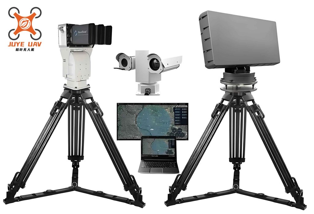
Key assumptions and parameters for this anti-UAV problem are defined as follows:
- Environment: A battlefield of dimensions \( L \) (length) \(\times\) \( W \) (width) \(\times\) \( H \) (height).
- Defenders (UGVs): \(n\) mobile units. Each UGV \(i\) has a position \(\mathbf{p}_i^{UGV}\), a constant velocity \(v_{UGV}\), a radar perception radius \(\rho_{radar}\), and a weapon with effective engagement range \([\rho_{min}, \rho_{max}]\), muzzle velocity \(v_0\), lethality \(\omega\), and a firing cooldown period \(t_{cool}\).
- Attackers (UAVs): \(m\) hostile UAVs. Each UAV \(j\) has a position \(\mathbf{p}_j^{UAV}\), a constant velocity \(v_{UAV}\) directed toward the asset, and a defensive capacity \(\xi\).
- Protected Asset: A stationary high-value site located within the environment.
- Goal: Maximize the number of UAVs destroyed while ensuring the asset’s survival. The mission fails if any UAV reaches the asset’s location.
The core challenge is to find the optimal dynamic policy for joint positioning and fire distribution among the UGVs to achieve this goal under time pressure and resource constraints, a quintessential problem in modern anti-UAV operations.
Methodological Framework: A Dec-POMDP Formulation
We model the collaborative anti-UAV task as a decentralized partially observable Markov decision process (Dec-POMDP), defined by the tuple \(G = \langle S, U, P, r, Z, O, n, \gamma \rangle\).
- \(s \in S\): The true global state of the environment.
- \(u^a \in U\): The action taken by agent \(a\). The joint action is \(\mathbf{u} \in \mathbf{U} \equiv U^n\).
- \(P(s’|s,\mathbf{u})\): The state transition function.
- \(r(s, \mathbf{u})\): The shared global reward function.
- \(z^a \in Z\): The local observation of agent \(a\), derived from \(O(s, a)\).
- \(\gamma\): The discount factor.
Each UGV is controlled by an independent agent. Following the centralised training with decentralised execution (CTDE) paradigm, agents have access to full state information during training but must rely solely on their local action-observation history \(\tau^a\) during execution. The joint policy \(\pi\) has a joint action-value function:
$$Q^\pi(s_t, \mathbf{u}_t) = \mathbb{E}_{s_{t+1:\infty}, \mathbf{u}_{t+1:\infty}} \left[ \sum_{i=0}^{\infty} \gamma^i r_{t+i} | s_t, \mathbf{u}_t \right]$$
1. State Space Design with Fused Situational Information
Effective decision-making in anti-UAV combat requires rich situational understanding. We design the observation space for each agent by fusing basic entity information with multi-source situational metrics.
Local Observation \(o_i\) for Agent \(i\): It consists of features for all entities (self, other UGVs, all UAVs, the asset). For an entity \(j\), the feature vector is populated only if it lies within the agent’s radar range \(\rho_{radar}\); otherwise, it is zeroed out.
$$d_{ij} = || \mathbf{p}_j – \mathbf{p}_i^{UGV} ||_2$$
$$o_{ij} = \begin{cases}
[\text{Basic Info}, \text{Situational Info}] & \text{if } d_{ij} \le \rho_{radar}\\
\mathbf{0} & \text{otherwise}
\end{cases}$$
$$o_i = [o_{i1}, o_{i2}, …, o_{i,(m+n+1)}]$$
Basic Information includes entity type, ID, position, velocity, and heading.
Situational Information is computed for each UAV target and provides a comprehensive threat and engagement picture. For a UAV target \(T\), we calculate a 5-dimensional vector \(S_T = [C_T, \rho_{far}, \rho_{near}, t_p, t_{target}]\):
- Threat Score (\(C_T\)): Calculated using a TOPSIS-based multi-attribute decision-making method. Let the feature matrix for \(m\) targets be \(X \in \mathbb{R}^{m \times 4} = [d_i, v_i, h_i, \beta_i]\), representing relative distance, relative velocity, height, and route shortcut. After normalization and weighting (using equal weights \(\mathbf{w} = [0.25, 0.25, 0.25, 0.25]\)), we find the positive and negative ideal solutions \(X^+\) and \(X^-\). The threat score is:
$$D^+_i = \sqrt{\sum_{k=1}^{4} w_k (X_{ik} – X^+_k)^2}, \quad D^-_i = \sqrt{\sum_{k=1}^{4} w_k (X_{ik} – X^-_k)^2}$$
$$C_i = \frac{D^-_i}{D^+_i + D^-_i + \epsilon}$$
where \(\epsilon=10^{-8}\) ensures numerical stability. A higher \(C_i\) indicates a greater threat. - Far Boundary (\(\rho_{far}\)) & Near Boundary (\(\rho_{near}\)): These dynamic boundaries define the effective launch area for a successful intercept, accounting for the projectile’s time-of-flight \(t_p\).
$$\rho_{far} = \sqrt{ \rho_{max}^2 + (v_{UAV} t_p)^2 + 2 v_{UAV} t_p \sqrt{\rho_{max}^2 – h^2 – \beta^2} }$$
$$\rho_{near} = \sqrt{ \rho_{min}^2 + (v_{UAV} t_p)^2 + 2 v_{UAV} t_p \sqrt{\rho_{min}^2 – h^2 – \beta^2} }$$
A target is kinematically engageable if its distance is within \([\rho_{near}, \rho_{far}]\). - Projectile Time-of-Flight (\(t_p\)): The estimated time for a shell to reach the predicted intercept point, solved via the ballistics equation.
- Time-to-Target (\(t_{target}\)): The estimated time for the UAV to reach the protected asset.
The global state \(s\) is the concatenation of all agents’ local observations, but with situational information calculated assuming perfect perception (i.e., \(\rho_{radar} \to \infty\)), used only during centralized training.
| Component | Description | Purpose |
|---|---|---|
| Basic Info | Type, ID, Position, Velocity, Heading | Provide fundamental entity tracking. |
| Threat Score (\(C_T\)) | Normalized score from 0 to 1. | Prioritize high-threat targets in anti-UAV engagement. |
| Engagement Boundaries (\(\rho_{far}, \rho_{near}\)) | Dynamic range limits for successful intercept. | Assess kinematic feasibility of a shot. |
| Temporal Metrics (\(t_p, t_{target}\)) | Projectile flight time and UAV time-to-target. | Enable time-sensitive decision-making. |
2. Action Space: Macro-Actions for Anti-UAV Engagement
Each UGV agent has a discrete action space \(A_i\) of dimension \(5 + m\):
$$A_i = \{\text{No-op}, \text{Move East}, \text{Move South}, \text{Move West}, \text{Move North}, \text{Fire at UAV}_1, …, \text{Fire at UAV}_m\}$$
The “Fire” actions are designed as macro-actions that encapsulate the complete firing sequence, which involves complex ballistics calculations:
- Trajectory Prediction & Intercept Point Calculation: Predict the UAV’s future position assuming constant velocity: \(\mathbf{p}_{predicted} = \mathbf{p}_{UAV} + \mathbf{v}_{UAV} \cdot t_p\).
- Ballistic Equation Solving: Compute the required time-of-flight \(t_p\) and elevation angle \(\alpha\). Let \(\Delta x, \Delta y, \Delta z\) be the relative coordinates from gun to predicted point, \(R = \sqrt{\Delta x^2 + \Delta z^2}\), and \(\theta = \arctan2(\Delta z, \Delta x)\). The flight time satisfies:
$$\frac{1}{4}g^2 t^4 + (g \Delta y – v_0^2) t^2 + (\Delta y^2 + R^2) = 0$$
This is solved numerically (e.g., Newton’s method). The elevation angle is then:
$$\alpha = \arcsin\left(\text{clip}\left( \frac{\Delta y + \frac{1}{2} g t^2}{v_0 t}, -1, 1 \right) \right)$$ - Trajectory Simulation & Damage Verification: The shell’s 3D initial velocity is \(\mathbf{v}_{initial} = [v_0 \cos\alpha \cos\theta, v_0 \sin\alpha, v_0 \cos\alpha \sin\theta]^T\). Its trajectory is simulated using Verlet integration over time step \(\Delta t\):
$$\mathbf{p}_{next} = \mathbf{p}_{current} + \mathbf{v}_{current} \Delta t + \frac{1}{2} \mathbf{a} (\Delta t)^2$$
$$\mathbf{v}_{next} = \mathbf{v}_{current} + \mathbf{a} \Delta t$$
where \(\mathbf{a} = [0, -g, 0]^T\). A hit is confirmed if the simulated shell passes within a lethal radius \(r_{damage}\) of the target. - Damage Probability Assessment: Upon a near detonation (proximity fuse), the kill probability \(p_{kill}\) is modeled based on fragment density \(\rho\):
$$\rho = \exp\left(-\frac{d^2}{2\sigma^2}\right), \quad p_{kill} = 1 – \exp(-\rho \lambda_0)$$
where \(d\) is the miss distance, \(\sigma\) controls spread, and \(\lambda_0\) is a lethality coefficient. A successful kill is determined by sampling \(p_{kill}\).
3. Hierarchical Multi-Objective Reward Function
A carefully structured reward function \(R\) is pivotal for guiding agents in this complex anti-UAV task. Our design incorporates five key mechanisms:
$$R = \underbrace{R_1 \cdot \mathbb{I}_{\{\text{first\_target}\}}}_{\text{Diversity}} + \underbrace{R_2 \cdot \mathbb{I}_{\{\text{fire\_action}\}}}_{\text{}} + \underbrace{\sum_{i=1}^{M} R_3 \cdot \frac{t_{current} + t^i_{fire}}{t^i_{flight}}}_{\text{Shaping}} + \underbrace{R_4 \cdot \Delta N_{kill}}_{\text{Success}} + \underbrace{R_5 \cdot \mathbb{I}_{\{\text{ammo\_save}\}}}_{\text{Efficiency}}$$
$$\quad – \underbrace{R_6 \cdot \mathbb{I}_{\{\text{out\_of\_bounds}\}}}_{\text{Safety}} – \underbrace{\sum_{j=1}^{n} R_7 \cdot \frac{1}{d_j}}_{\text{}} + \underbrace{R_8 \cdot \mathbb{I}_{\{\text{success}\}} – R_9 \cdot \mathbb{I}_{\{\text{fail}\}}}_{\text{Global Outcome}}$$
1. Diversity Encouragement: \(R_1\) is awarded for the first time a specific UAV is targeted, promoting target variety and preventing fixation. Subsequent locks on the same target receive a smaller \(R_2\).
2. Temporal Credit Assignment & Shaping: To address the delay between firing and hit (fire control delay), a pre-reward proportional to \((t_{current}+t_{fire})/t_{flight}\) is given for each shell in flight. This provides incremental feedback, mitigating sparse rewards. A final kill confirmation reward \(R_4\) is granted upon target destruction.
3. Resource Efficiency: A bonus \(R_5\) is given for “precise” shots where the calculated kill probability \(p_{kill}\) exceeds a high threshold, encouraging ammunition conservation.
4. Behavioral Constraints: Penalties are imposed for moving out of bounds (\(-R_6\)) and for collisions between UGVs (\(-R_7/d_j\), where \(d_j\) is distance to the nearest ally).
5. Global Mission Outcome: A large positive reward \(R_8\) is given for mission success (all UAVs destroyed), and a large negative penalty \(-R_9\) is given for mission failure (asset destroyed).
| Component | Mathematical Form | Primary Objective |
|---|---|---|
| Diversity Reward | \(R_1, R_2\) | Encourage engaging multiple UAVs. |
| Temporal Shaping | \(R_3 \cdot \frac{t_{current}+t_{fire}}{t_{flight}}\) | Provide intermediate feedback for delayed outcomes. |
| Kill Confirmation | \(R_4 \cdot \Delta N_{kill}\) | Reinforce successful anti-UAV kills. |
| Efficiency Bonus | \(R_5 \cdot \mathbb{I}_{\{p_{kill} > \theta\}}\) | Promote ammunition-efficient shots. |
| Boundary Penalty | \(-R_6\) | Keep UGVs within valid operation area. |
| Collision Penalty | \(-R_7 / d\) | Maintain safe separation between friendly units. |
| Global Outcome | \(+R_8 / -R_9\) | Strongly align policy with ultimate mission success/failure. |
4. Training with Monotonic Value Decomposition
We adopt the QMIX algorithm for training our multi-agent anti-UAV system. QMIX enforces a monotonicity constraint between individual agent utilities \(Q_a(\tau^a, u^a)\) and the joint action-value \(Q_{tot}(\boldsymbol{\tau}, \mathbf{u})\):
$$Q_{tot}(\boldsymbol{\tau}, \mathbf{u}) = f_s\left(Q_1(\tau^1, u^1), …, Q_n(\tau^n, u^n)\right) \quad \text{with} \quad \frac{\partial f_s}{\partial Q_a} \geq 0, \forall a$$
Here, \(f_s\) is a mixing network whose non-negative weights are generated by hypernetworks conditioned on the global state \(s\). This structure allows for centralized learning of complex cooperative value functions while enabling decentralized execution via argmax operations on individual \(Q_a\) networks. Training minimizes the TD error on samples from a replay buffer:
$$\mathcal{L}(\theta) = \sum_{b} \left( Q_{tot}(s, \mathbf{u}; \theta) – y \right)^2, \quad y = r + \gamma \max_{\mathbf{u}’} Q_{tot}(s’, \mathbf{u}’; \theta^-)$$
where \(\theta^-\) are the parameters of a target network.
Experimental Analysis and Results
We constructed a simulation environment based on the defined anti-UAV scenario to validate our approach, termed Situational-Fused Hierarchical Multi-Objective Multi-agent RL (SF-HIMO).
Experimental Setup
Scenarios: Three distinct anti-UAV challenge scenarios were designed:
- Attack_South: 10 UAVs attack from random southern positions.
- Attack_Four: 10 UAVs attack from random positions on all four sides.
- Attack_Large: A scaled-up scenario with 6 UGVs defending against 30 UAVs attacking from four sides.
System Parameters: The battlefield is 8km x 8km. Key parameters are summarized below.
| Entity | Parameter | Value |
|---|---|---|
| UGV (Defender) | Number (Attack_South/Four) | 3 |
| Number (Attack_Large) | 6 | |
| Speed \(v_{UGV}\) | 10 m/s | |
| Weapon Range \([\rho_{min}, \rho_{max}]\) | [700m, 2500m] | |
| Firing Cooldown \(t_{cool}\) | 2 s | |
| Muzzle Velocity \(v_0\) | 1050 m/s | |
| UAV (Attacker) | Speed \(v_{UAV}\) | 60 m/s |
| Defensive Capacity \(\xi\) | 60 | |
| Value | 1 | |
| Projectile | Lethal Radius \(r_{damage}\) | 15 m |
| Fragment Spread \(\sigma\) | 5 | |
| Lethality Coefficient \(\lambda_0\) | 1.6 |
Baselines & Evaluation: We compared SF-HIMO against three prominent MADRL algorithms: Finetuned-QMIX, QPLEX, and QTRAN. The primary metric is the average mission success rate (win %) over the final testing episodes. All results are averaged over multiple random seeds.
Performance Results
The quantitative results demonstrate the superiority of our SF-HIMO framework in all tested anti-UAV scenarios.
| Scenario | SF-HIMO (Ours) | Finetuned-QMIX | QPLEX | QTRAN |
|---|---|---|---|---|
| Attack_South | 86% ± 3% | 34% ± 4% | 29% ± 8% | 0% |
| Attack_Four | 88% ± 3% | 72% ± 4% | 69% ± 7% | 0% |
| Attack_Large | 78% ± 4% | 69% ± 7% | 43% ± 6% | 0% |
SF-HIMO achieves an average performance improvement of 48.9% over the baseline algorithms. Notably, it excels in the more challenging Attack_South scenario, where targets are densely clustered, showcasing its enhanced ability to manage contention and coordinate fire. The algorithm also maintains high effectiveness in the large-scale scenario, proving its scalability. QTRAN failed to learn an effective policy in this complex domain, highlighting the non-trivial nature of the anti-UAV problem.
Ablation Studies
To dissect the contribution of our core innovations, we conducted ablation studies on the two main components of SF-HIMO.
- SF-HIMO_MR: Removes the hierarchical multi-objective reward, using only basic kill/failure/collision rewards.
- SF-HIMO_MS: Removes the multi-source situational information from the state space.
- Finetuned-QMIX: The base algorithm without both situational information and the advanced reward.
| Scenario | SF-HIMO (Full) | SF-HIMO_MR | SF-HIMO_MS | Finetuned-QMIX |
|---|---|---|---|---|
| Attack_South | 86% | 73% | 45% | 34% |
| Attack_Four | 88% | 85% | 73% | 72% |
The results confirm that both proposed components are essential and complementary. The performance drop is more severe when situational information is removed (SF-HIMO_MS), particularly in the complex Attack_South scenario. This underscores the critical role of fused situational awareness—threat assessment, engagement boundaries, temporal metrics—in enabling intelligent anti-UAV decision-making. The hierarchical reward (SF-HIMO_MR) also provides a significant boost, especially in shaping behavior for long-delay outcomes and efficient resource use.
Conclusion
This work presents a novel and effective intelligent framework for artillery-based anti-UAV defense. By formulating the problem as a cooperative multi-agent task and developing the SF-HIMO algorithm, we address key limitations of traditional systems. The integration of multi-source situational information directly into the agent’s observation space provides a comprehensive and actionable understanding of the dynamic battlefield, crucial for effective anti-UAV operations. Furthermore, the carefully designed hierarchical multi-objective reward function successfully guides the learning process, balancing immediate feedback with long-term strategic goals, encouraging efficient behavior, and enforcing safety constraints.
Extensive simulation experiments across diverse and challenging anti-UAV scenarios demonstrate that our framework significantly outperforms state-of-the-art multi-agent reinforcement learning baselines, achieving markedly higher mission success rates and robust scalability. The ablation studies provide clear evidence for the necessity and synergy of its core components. This research offers a promising pathway toward deploying adaptive, efficient, and intelligent autonomous systems for countering the growing threat of UAV swarms, marking a substantial step forward in the evolution of modern anti-UAV warfare technology.