
In recent years, the rapid advancement of unmanned aerial vehicle (UAV) technology, particularly small and micro-UAVs, has led to their widespread use in both civilian and military domains. These UAVs possess characteristics such as stealth capabilities, ease of operation, strong penetration abilities, diverse acquisition channels, and flexible deployment modes, enabling them to effectively execute missions like harassment, reconnaissance, strikes, and assessment. This has significantly increased their military applications. For instance, in early 2018, Russia’s Khmeimim Air Base and Tartus Naval Base in Syria faced attacks from a swarm of UAVs, which were successfully countered using the “Pantsir-S” air defense system and electronic warfare measures. Similarly, the 2020 Nagorno-Karabakh conflict highlighted the devastating impact of UAVs in modern warfare, drawing global attention to anti-UAV operations. As a result, major military powers worldwide are actively researching methods to counter UAV threats, with a focus on small and micro-UAVs. The detection and reconnaissance of these UAVs are critical starting points in anti-UAV operations, yet they remain a challenging aspect due to the technical limitations of existing systems. Typically, a composite approach involving multiple detection methods—such as radar, radio frequency monitoring, and electro-optical systems—networked together is required to achieve effective reconnaissance intelligence in anti-UAV scenarios. Evaluating the operational effectiveness of such reconnaissance intelligence systems is essential for understanding their performance, optimizing their deployment, and informing tactical decisions. In this article, I will explore the operational effectiveness evaluation of anti-UAV reconnaissance intelligence systems, focusing on the construction of an evaluation index system and the application of analytical methods like the Analytic Hierarchy Process (AHP) and fuzzy comprehensive evaluation. I will also incorporate tables and formulas to summarize key points, ensuring a comprehensive analysis that exceeds 8000 tokens in length.
The anti-UAV reconnaissance intelligence system primarily comprises several capability subsystems, including radar detection, radio frequency monitoring, and electro-optical detection. Each subsystem plays a distinct role in identifying and tracking UAVs. Radio frequency monitoring is a passive detection method that relies on intercepting remote control and telemetry signals from UAVs to detect and determine their direction. This approach offers advantages like stealth and low exposure, but it fails when UAVs operate in radio-silent modes. Key functions include frequency measurement, direction finding, and, when used in groups, locating UAV operators. Radar detection, on the other hand, provides all-weather operation with high accuracy and stability, though it may struggle with targets having low radial velocities. It enables functions such as positioning, speed measurement, distance measurement, and multi-target tracking for small UAVs. Electro-optical detection utilizes visible and near-infrared electromagnetic waves: visible light detection works by imaging reflected light from UAVs, similar to human vision, while near-infrared detection leverages the thermal radiation from UAV motors for tracking. Integrating these subsystems into a networked system enhances overall anti-UAV capabilities, but assessing their combined effectiveness requires a structured evaluation framework. Below, I will insert an image that visually represents the complexity of anti-UAV systems, highlighting the integration of various detection technologies.
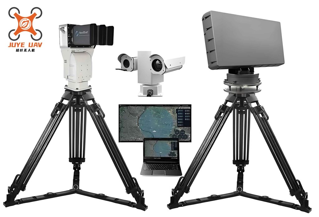
To evaluate the operational effectiveness of an anti-UAV reconnaissance intelligence system, I first construct an evaluation index system based on its operational missions and primary functions. This system must reflect the key performance indicators that influence overall effectiveness, adhering to principles of systematic organization, hierarchical structure, and quantifiability. The process involves decomposing the system’s capabilities into specific performance metrics, then selecting those that significantly impact operational outcomes. For radio frequency monitoring capability, critical indicators include monitoring frequency range, direction-finding accuracy, frequency measurement accuracy, and response time. Radar detection capability relies on indicators such as detection range, detection probability, azimuth measurement accuracy, elevation measurement accuracy, number of simultaneously tracked targets, and detectable target speed range. Electro-optical detection capability depends on tracking angular velocity range, tracking accuracy, laser ranging accuracy, and system response time. By consolidating these, I establish a hierarchical index system with three primary indicators and fourteen secondary indicators, as summarized in the table below.
| Primary Indicators | Secondary Indicators | Description |
|---|---|---|
| Radio Frequency Monitoring | Monitoring Frequency Range (U11) | The range of frequencies the system can monitor for UAV signals. |
| Direction-Finding Accuracy (U12) | Precision in determining the direction of UAV signals. | |
| Frequency Measurement Accuracy (U13) | Accuracy in measuring the frequency of intercepted signals. | |
| Response Time (U14) | Time taken to detect and process signals. | |
| Radar Detection | Detection Range (U21) | Maximum distance at which UAVs can be detected. |
| Detection Probability (U22) | Likelihood of successfully detecting a UAV within range. | |
| Azimuth Measurement Accuracy (U23) | Accuracy in measuring horizontal angle of UAVs. | |
| Elevation Measurement Accuracy (U24) | Accuracy in measuring vertical angle of UAVs. | |
| Simultaneously Tracked Targets (U25) | Number of UAVs the radar can track at once. | |
| Detectable Speed Range (U26) | Range of UAV speeds that can be detected. | |
| Electro-Optical Detection | Tracking Angular Velocity Range (U31) | Range of angular velocities the system can track. |
| Tracking Accuracy (U32) | Precision in tracking UAV movements. | |
| Laser Ranging Accuracy (U33) | Accuracy of distance measurements using lasers. | |
| Response Time (U34) | Time taken to acquire and process electro-optical data. |
With the index system in place, I proceed to develop an evaluation model using the Analytic Hierarchy Process (AHP) and fuzzy comprehensive evaluation. AHP is employed to determine the weights of each indicator, reflecting their relative importance in anti-UAV operations. This involves two levels: single-level sorting, which compares indicators within the same hierarchical level, and total-level sorting, which assesses all bottom-level indicators against the overall goal. To construct judgment matrices, I use a 9-point scale where values from 1 to 9 represent the importance of one indicator relative to another, as shown in Table 2. Experts in anti-UAV systems provide pairwise comparisons based on their experience, ensuring the matrices capture realistic priorities.
| Scale Value | Interpretation |
|---|---|
| 1 | Equal importance |
| 3 | Slightly more important |
| 5 | Clearly more important |
| 7 | Strongly more important |
| 9 | Extremely more important |
| 1/3, 1/5, 1/7, 1/9 | Reciprocals for less importance |
For example, let the judgment matrix for the three primary indicators—Radio Frequency Monitoring (A1), Radar Detection (A2), and Electro-Optical Detection (A3)—be denoted as \( B_0 \). Based on expert input, I define \( B_0 \) as follows:
$$ B_0 = \begin{bmatrix} 1 & 1/3 & 3 \\ 3 & 1 & 5 \\ 1/3 & 1/5 & 1 \end{bmatrix} $$
To calculate the weights, I use the root method. First, compute the product of each row:
$$ M_i = \prod_{j=1}^{n} a_{ij} \quad \text{for} \quad i = 1, 2, \ldots, n $$
For \( B_0 \), with \( n = 3 \):
$$ M_1 = 1 \times 1/3 \times 3 = 1, \quad M_2 = 3 \times 1 \times 5 = 15, \quad M_3 = 1/3 \times 1/5 \times 1 = 1/15 $$
Next, compute the \( n \)-th root of each \( M_i \):
$$ W_i = \sqrt[n]{M_i} $$
Thus:
$$ W_1 = \sqrt[3]{1} = 1, \quad W_2 = \sqrt[3]{15} \approx 2.466, \quad W_3 = \sqrt[3]{1/15} \approx 0.405 $$
Then, normalize the vector \( \mathbf{W} = [W_1, W_2, W_3]^T \):
$$ \sum_{j=1}^{3} W_j = 1 + 2.466 + 0.405 = 3.871 $$
The normalized weights are:
$$ w_1 = \frac{1}{3.871} \approx 0.258, \quad w_2 = \frac{2.466}{3.871} \approx 0.637, \quad w_3 = \frac{0.405}{3.871} \approx 0.105 $$
So, the weight vector for primary indicators is \( \mathbf{W}_0 = [0.258, 0.637, 0.105]^T \). To ensure consistency, I calculate the maximum eigenvalue \( \lambda_{\text{max}} \) using:
$$ \lambda_{\text{max}} = \sum_{i=1}^{n} \frac{(A\mathbf{W})_i}{nW_i} $$
Where \( A \) is the judgment matrix. For \( B_0 \), compute \( A\mathbf{W} \):
$$ A\mathbf{W} = \begin{bmatrix} 1 & 1/3 & 3 \\ 3 & 1 & 5 \\ 1/3 & 1/5 & 1 \end{bmatrix} \begin{bmatrix} 0.258 \\ 0.637 \\ 0.105 \end{bmatrix} = \begin{bmatrix} 0.258 + 0.212 + 0.315 \\ 0.774 + 0.637 + 0.525 \\ 0.086 + 0.127 + 0.105 \end{bmatrix} = \begin{bmatrix} 0.785 \\ 1.936 \\ 0.318 \end{bmatrix} $$
Then:
$$ \lambda_{\text{max}} = \frac{0.785}{3 \times 0.258} + \frac{1.936}{3 \times 0.637} + \frac{0.318}{3 \times 0.105} = \frac{0.785}{0.774} + \frac{1.936}{1.911} + \frac{0.318}{0.315} \approx 1.014 + 1.013 + 1.010 = 3.037 $$
The consistency index (CI) is given by:
$$ CI = \frac{\lambda_{\text{max}} – n}{n – 1} = \frac{3.037 – 3}{2} = 0.0185 $$
For \( n = 3 \), the random index (RI) is 0.58. The consistency ratio (CR) is:
$$ CR = \frac{CI}{RI} = \frac{0.0185}{0.58} \approx 0.0319 $$
Since \( CR < 0.1 \), the matrix \( B_0 \) is consistent. Similarly, I construct judgment matrices for the secondary indicators under each primary indicator. For Radio Frequency Monitoring (A1), with secondary indicators U11, U12, U13, U14, the judgment matrix \( B_1 \) is:
$$ B_1 = \begin{bmatrix} 1 & 3 & 5 & 3 \\ 1/3 & 1 & 3 & 3 \\ 1/5 & 1/3 & 1 & 2 \\ 1/3 & 1/3 & 1/2 & 1 \end{bmatrix} $$
Following the same root method, the weight vector for \( B_1 \) is computed as \( \mathbf{W}_1 = [0.519, 0.263, 0.121, 0.097]^T \), with \( \lambda_{\text{max}} \approx 4.233 \), \( CI \approx 0.074 \), and \( CR \approx 0.082 \) (using RI = 0.90 for n=4), indicating consistency. For Radar Detection (A2), with six secondary indicators U21 to U26, the judgment matrix \( B_2 \) is:
$$ B_2 = \begin{bmatrix} 1 & 3 & 5 & 7 & 3 & 1/2 \\ 1/3 & 1 & 3 & 3 & 3 & 1/5 \\ 1/5 & 1/3 & 1 & 3 & 3 & 1/7 \\ 1/7 & 1/3 & 1/3 & 1 & 3 & 1/5 \\ 1/3 & 1/3 & 1/3 & 1/3 & 1 & 1/7 \\ 2 & 5 & 7 & 5 & 7 & 1 \end{bmatrix} $$
The weight vector is \( \mathbf{W}_2 = [0.273, 0.128, 0.081, 0.057, 0.043, 0.418]^T \), with \( \lambda_{\text{max}} \approx 6.61 \), \( CI \approx 0.122 \), and \( CR \approx 0.098 \) (RI = 1.24 for n=6). For Electro-Optical Detection (A3), with secondary indicators U31 to U34, the judgment matrix \( B_3 \) is:
$$ B_3 = \begin{bmatrix} 1 & 3 & 3 & 1/3 \\ 1/3 & 1 & 3 & 1/3 \\ 1/3 & 1/3 & 1 & 1/7 \\ 3 & 3 & 7 & 1 \end{bmatrix} $$
The weight vector is \( \mathbf{W}_3 = [0.257, 0.146, 0.067, 0.530]^T \), with \( \lambda_{\text{max}} \approx 4.162 \), \( CI \approx 0.054 \), and \( CR \approx 0.060 \). Next, I perform total-level sorting to obtain the weights of all fourteen secondary indicators relative to the overall goal. The weight \( w_i \) for indicator \( i \) is calculated as:
$$ w_i = w_{\text{primary}} \times w_{\text{secondary}} $$
Where \( w_{\text{primary}} \) is the weight of the primary indicator, and \( w_{\text{secondary}} \) is the weight within that primary indicator. The resulting weight vector \( \mathbf{W} \) for all secondary indicators is:
$$ \mathbf{W} = [0.134, 0.068, 0.031, 0.025, 0.174, 0.082, 0.052, 0.036, 0.027, 0.266, 0.027, 0.015, 0.007, 0.056] $$
These weights reflect the relative importance of each indicator in anti-UAV reconnaissance intelligence systems, with higher values indicating greater impact on operational effectiveness.
After determining the weights, I apply the fuzzy comprehensive evaluation method to assess the operational effectiveness. This approach handles the vagueness and uncertainty in evaluating anti-UAV systems, as performance levels are often subjective and context-dependent. First, I define the factor set \( U \) containing all fourteen secondary indicators:
$$ U = \{ u_1, u_2, \ldots, u_{14} \} $$
Next, I establish an evaluation set \( V \) with five levels:
$$ V = \{ \text{Excellent}, \text{Good}, \text{Moderate}, \text{Poor}, \text{Very Poor} \} $$
For each indicator, experts or system users provide ratings based on their experience. For example, for indicator U11 (Monitoring Frequency Range), suppose six evaluators assign the following membership degrees across the five levels: 30% Excellent, 50% Good, 10% Moderate, 10% Poor, and 0% Very Poor. This forms a fuzzy evaluation matrix \( D_{11} \):
$$ D_{11} = \begin{bmatrix} 0.3 & 0.5 & 0.1 & 0.1 & 0 \\ 0.2 & 0.4 & 0.2 & 0.2 & 0 \\ 0.2 & 0.5 & 0.2 & 0.1 & 0 \\ 0.1 & 0.4 & 0.3 & 0.1 & 0.1 \\ 0.2 & 0.3 & 0.3 & 0.1 & 0.1 \\ 0.2 & 0.4 & 0.2 & 0.1 & 0.1 \end{bmatrix} $$
To derive the overall fuzzy evaluation vector for U11, I average the columns:
$$ r_{11} = \frac{1}{6} \sum_{i=1}^{6} d_{i1} = \frac{0.3+0.2+0.2+0.1+0.2+0.2}{6} = \frac{1.2}{6} = 0.200 $$
$$ r_{12} = \frac{0.5+0.4+0.5+0.4+0.3+0.4}{6} = \frac{2.5}{6} \approx 0.417 $$
$$ r_{13} = \frac{0.1+0.2+0.2+0.3+0.3+0.2}{6} = \frac{1.3}{6} \approx 0.217 $$
$$ r_{14} = \frac{0.1+0.2+0.1+0.1+0.1+0.1}{6} = \frac{0.7}{6} \approx 0.117 $$
$$ r_{15} = \frac{0+0+0+0.1+0.1+0.1}{6} = \frac{0.3}{6} = 0.050 $$
Thus, the fuzzy evaluation vector for U11 is \( \mathbf{R}_{11} = [0.200, 0.417, 0.217, 0.117, 0.050] \). Repeating this process for all indicators, I compile the overall fuzzy evaluation matrix \( \mathbf{R} \). For brevity, assume the following matrix based on expert assessments for anti-UAV systems:
$$ \mathbf{R} = \begin{bmatrix} 0.183 & 0.433 & 0.217 & 0.117 & 0.050 \\ 0.236 & 0.281 & 0.384 & 0.060 & 0.039 \\ 0.132 & 0.352 & 0.352 & 0.132 & 0.032 \\ 0.117 & 0.217 & 0.421 & 0.132 & 0.113 \\ 0.167 & 0.342 & 0.183 & 0.217 & 0.091 \\ 0.352 & 0.433 & 0.117 & 0.098 & 0.000 \\ 0.217 & 0.433 & 0.217 & 0.133 & 0.000 \\ 0.117 & 0.217 & 0.183 & 0.433 & 0.050 \\ 0.433 & 0.312 & 0.217 & 0.038 & 0.000 \\ 0.217 & 0.321 & 0.352 & 0.050 & 0.050 \\ 0.256 & 0.433 & 0.126 & 0.106 & 0.079 \\ 0.351 & 0.238 & 0.316 & 0.095 & 0.000 \\ 0.237 & 0.281 & 0.196 & 0.206 & 0.080 \\ 0.033 & 0.317 & 0.217 & 0.117 & 0.316 \end{bmatrix} $$
Now, I compute the comprehensive evaluation vector \( \mathbf{E} \) by multiplying the weight vector \( \mathbf{W} \) with the matrix \( \mathbf{R} \):
$$ \mathbf{E} = \mathbf{W} \cdot \mathbf{R} $$
This involves a weighted sum. For each level in \( V \), calculate:
$$ e_j = \sum_{i=1}^{14} w_i \cdot r_{ij} \quad \text{for} \quad j = 1, 2, \ldots, 5 $$
Performing the calculations:
$$ e_1 = 0.134 \times 0.183 + 0.068 \times 0.236 + \ldots + 0.056 \times 0.033 \approx 0.206 $$
$$ e_2 = 0.134 \times 0.433 + 0.068 \times 0.281 + \ldots + 0.056 \times 0.317 \approx 0.349 $$
$$ e_3 = 0.134 \times 0.217 + 0.068 \times 0.384 + \ldots + 0.056 \times 0.217 \approx 0.257 $$
$$ e_4 = 0.134 \times 0.117 + 0.068 \times 0.060 + \ldots + 0.056 \times 0.117 \approx 0.126 $$
$$ e_5 = 0.134 \times 0.050 + 0.068 \times 0.039 + \ldots + 0.056 \times 0.316 \approx 0.063 $$
Thus, \( \mathbf{E} = [0.206, 0.349, 0.257, 0.126, 0.063] \). This result indicates the membership degrees of the anti-UAV reconnaissance intelligence system’s operational effectiveness across the five levels. According to the maximum membership principle, the highest value is 0.349 for “Good,” suggesting that the overall effectiveness is rated as Good. However, the combined membership for “Excellent” and “Good” is \( 0.206 + 0.349 = 0.555 \), or 55.5%, which underscores a moderately positive evaluation but also highlights areas for improvement in anti-UAV capabilities.
To further analyze the results, I discuss the implications for anti-UAV operations. The evaluation reveals that radar detection contributes significantly to overall effectiveness, given its high weight in the index system. This aligns with the critical role of radar in detecting small UAVs across various environments. Conversely, electro-optical detection, while important, shows lower weights for some indicators, suggesting that enhancements in tracking accuracy and response time could boost anti-UAV performance. The fuzzy comprehensive evaluation effectively captures the subjective nature of expert assessments, allowing for a nuanced understanding of system strengths and weaknesses. In practice, this evaluation can guide decision-makers in optimizing anti-UAV strategies, such as allocating resources to improve specific subsystems or integrating new technologies. For instance, advancing radio frequency monitoring to handle radio-silent UAVs or enhancing radar algorithms for low-velocity targets could address current limitations. Moreover, the networked approach of combining multiple detection methods is validated by the evaluation, as it mitigates individual subsystem flaws and enhances overall robustness in anti-UAV missions.
In conclusion, the operational effectiveness evaluation of anti-UAV reconnaissance intelligence systems is a complex yet vital process for modern defense. By constructing a hierarchical index system and applying AHP and fuzzy comprehensive evaluation, I have demonstrated a structured method that combines qualitative and quantitative analysis. This approach offers clear logic, strong operability, and interpretable results, making it accessible for decision-makers in anti-UAV operations. The instance analysis illustrates how weights and fuzzy ratings can be derived to assess overall effectiveness, with results indicating a “Good” performance level. Future work could involve refining the indicators based on evolving anti-UAV technologies, incorporating real-time data from field tests, or expanding the evaluation to include cost-effectiveness analysis. Ultimately, continuous assessment and adaptation are key to staying ahead in the escalating challenge of countering UAV threats, ensuring that anti-UAV systems remain effective in diverse operational scenarios.