
Accurately forecasting the development cost of a military UAV is a critical challenge faced by defense agencies and aerospace contractors worldwide. These advanced systems represent a significant financial investment, with their unit-cost-per-mass often exceeding that of manned aircraft. The development expenditure not only dictates the initial acquisition feasibility but also has profound downstream implications for the system’s operational capabilities and long-term maintenance budget. Consequently, robust cost prediction models are essential tools for program planning, budgeting, and trade-off analysis during the early conceptual and design phases of a military UAV project.
The core difficulty in constructing such models lies in the characteristic “small sample, many variables” problem inherent to this domain. Detailed historical cost data for military UAV programs is scarce, often classified, and pertains to systems with vastly different missions and technological generations. Simultaneously, a wide array of technical parameters—such as airframe dimensions, propulsion performance, avionics sophistication, and mission profile metrics—are posited as potential cost drivers. This combination of limited data and a complex, potentially intercorrelated set of explanatory variables renders traditional statistical methods like Ordinary Least Squares (OLS) regression ineffective, as they suffer from multicollinearity and overfitting.
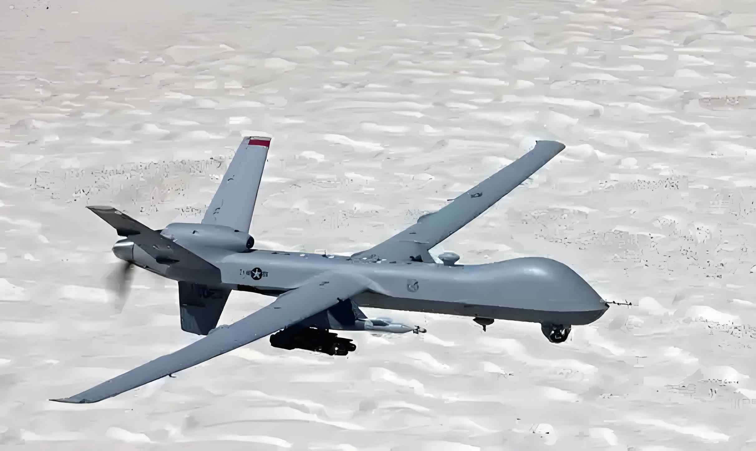
Existing approaches to military UAV cost estimation, including engineering buildup, analogy, and various parametric techniques, each have limitations. For preliminary design stages, parametric methods are most relevant. Techniques like Partial Least Squares (PLS) regression and Artificial Neural Networks (ANNs) have been explored. PLS handles collinearity but can be sensitive to model structure, while ANNs (like BP or RBF networks) require substantial data to train effectively and avoid local minima, a luxury rarely available in the military UAV domain. There is a clear need for a method that can extract the most salient cost drivers from a small set of historical military UAV projects while rigorously managing information redundancy among the candidate parameters.
This work proposes and demonstrates the application of Gram-Schmidt (G-S) regression for predicting the development cost of a military UAV. The Gram-Schmidt process is a classical orthogonalization technique that transforms a set of linearly independent vectors into an orthogonal set. When applied within a stepwise regression framework, it provides a powerful mechanism for variable selection and model building in the presence of multicollinearity and limited samples. The method sequentially identifies the parameter that explains the most variance in the cost variable, orthogonalizes the remaining candidates with respect to the selected one, and repeats the process. This ensures that each new variable entered into the model contributes unique, non-redundant explanatory power.
The fundamental mathematical procedure of Gram-Schmidt orthogonalization is as follows. Given a set of linearly independent predictor variables \( x_1, x_2, …, x_s \), we can construct an orthogonal set \( z_1, z_2, …, z_s \) using the iterative scheme:
$$
z_1 = x_1,
$$
$$
z_2 = x_2 – \frac{x_2^T z_1}{z_1^T z_1} z_1,
$$
$$
z_3 = x_3 – \frac{x_3^T z_1}{z_1^T z_1} z_1 – \frac{x_3^T z_2}{z_2^T z_2} z_2,
$$
$$
\vdots
$$
$$
z_s = x_s – \sum_{k=1}^{s-1} \frac{x_s^T z_k}{z_k^T z_k} z_k.
$$
In matrix form, the relationship between the original variables \( \mathbf{X} = (x_1, x_2, …, x_s) \) and the orthogonalized variables \( \mathbf{Z} = (z_1, z_2, …, z_s) \) is given by \( \mathbf{Z} = \mathbf{X} \mathbf{R}^{-1} \), where \( \mathbf{R} \) is an upper triangular matrix with ones on the diagonal. The coefficients \( r_{jk} \) are precisely the projection terms \( \frac{x_k^T z_j}{z_j^T z_j} \). For numerical stability, especially with highly correlated variables, a modified Gram-Schmidt algorithm is recommended, which updates vectors sequentially to minimize round-off error accumulation.
The stepwise Gram-Schmidt regression algorithm for military UAV cost prediction proceeds as follows, starting with a centered dataset where each predictor variable and the cost variable have a mean of zero:
- Initialization: Let \( z_{1j} = x_j \) for \( j = 1, 2, …, s \). Perform simple linear regression of the development cost \( Y \) on each \( z_{1j} \). Select the variable \( x_{p1} \) corresponding to the \( z_{1j} \) with the largest absolute t-statistic that exceeds the critical value. Set \( z_1 = x_{p1} \).
- Iterative Selection & Orthogonalization: For step \( m \) (where \( m \) starts at 1), generate new candidate variables for all predictors \( x_j \) not yet in the model:
$$ z_{(m+1)j} = x_j – \sum_{k=1}^{m} \frac{x_j^T z_k}{z_k^T z_k} z_k $$
(using the modified algorithm for stability). Regress \( Y \) on \( z_1, z_2, …, z_m, z_{(m+1)j} \) and evaluate the t-statistic for \( z_{(m+1)j} \). Select the variable \( x_{p(m+1)} \) corresponding to the candidate with the largest significant |t|. Set \( z_{m+1} = z_{(m+1)p} \). - Termination: Repeat Step 2 until no remaining orthogonalized candidate variable produces a significant t-statistic.
- Model Formulation: The final model is expressed in terms of the orthogonal components:
$$ Y = \beta_0 + \beta_1 z_1 + \beta_2 z_2 + … + \beta_q z_q $$
where \( q \) is the number of selected variables. Using the inverse transformation \( \mathbf{Z} = \mathbf{X} \mathbf{R}^{-1} \), this model is converted back to a function of the original, interpretable military UAV parameters \( x_{p1}, x_{p2}, …, x_{pq} \):
$$ \hat{y} = a_0 + a_1 x_{p1} + a_2 x_{p2} + … + a_q x_{pq}. $$
To illustrate this methodology, we consider a dataset from literature concerning the development cost of several historical military UAV systems. The candidate technical parameters are: Length (\(x_1\)), Maximum Take-Off Weight (\(x_2\)), Cruise Speed (\(x_3\)), Flight Altitude (\(x_4\)), Endurance (\(x_5\)), and Payload (\(x_6\)). The development cost (\(y\)) is the target variable. Data for six systems (A-F) serve as the training set, and one system (K) is held out for validation. All costs are normalized to a common fiscal year.
The correlation matrix (Table 1) for the training data immediately reveals the challenge. Strong interdependencies exist among nearly all technical parameters, confirming the presence of significant multicollinearity that would plague a standard OLS approach for military UAV cost estimation.
| Variable | \(x_1\) | \(x_2\) | \(x_3\) | \(x_4\) | \(x_5\) | \(x_6\) | \(y\) |
|---|---|---|---|---|---|---|---|
| \(x_1\) | 1.0000 | ||||||
| \(x_2\) | 0.9588 | 1.0000 | |||||
| \(x_3\) | 0.7256 | 0.8216 | 1.0000 | ||||
| \(x_4\) | 0.8447 | 0.9447 | 0.9417 | 1.0000 | |||
| \(x_5\) | 0.9819 | 0.9811 | 0.7881 | 0.9010 | 1.0000 | ||
| \(x_6\) | 0.9187 | 0.9841 | 0.8964 | 0.9743 | 0.9658 | 1.0000 | |
| \(y\) | 0.9145 | 0.9658 | 0.9131 | 0.9828 | 0.9522 | 0.9800 | 1.0000 |
Applying the Gram-Schmidt regression procedure to the centered training data (Table 2), the algorithm first identifies Flight Altitude (\(x_4\)) as the most significant individual predictor (\(z_1\)). After orthogonalizing the remaining variables with respect to \(z_1\), Length (\(x_1\)) emerges as the next most significant, providing unique explanatory power. No other orthogonalized variable passes the significance threshold for entry into the model.
| UAV | \(\tilde{x}_1\) | \(\tilde{x}_2\) | \(\tilde{x}_3\) | \(\tilde{x}_4\) | \(\tilde{x}_5\) | \(\tilde{x}_6\) | \(\tilde{y}\) |
|---|---|---|---|---|---|---|---|
| A | 6.15 | 7625 | 206.6 | 9.41 | 19.71 | 504.5 | 1.436 |
| B | -2.10 | -3517 | -44.43 | -6.39 | -15.29 | -265.5 | -0.944 |
| C | -5.27 | -3837 | -132.4 | -6.39 | -18.29 | -230.5 | -1.324 |
| D | -3.08 | -3597 | -320.4 | -8.39 | -17.29 | -381.0 | -1.254 |
| E | 6.15 | 6398 | 297.6 | 10.01 | 23.71 | 509.5 | 1.916 |
| F | -2.75 | -96.7 | 204.6 | 4.81 | -10.29 | 54.5 | 0.376 |
The resulting model in the orthogonal space is:
$$ \tilde{Y} = 0.1639z_1 + 0.0837z_2 $$
Transforming back to the original military UAV parameters yields the final cost prediction equation:
$$ \hat{y} = 0.371 + 0.0837x_1 + 0.1225x_4 $$
This remarkably parsimonious model, using only Flight Altitude and Length, achieves a coefficient of determination \(R^2 = 0.991\) on the training data. The model’s fit to the historical military UAV development costs is excellent, as shown in Table 3, with a maximum training error of 8.9% and a minimum of 1.2%.
| Training UAV | Actual Cost ($B) | Predicted Cost ($B) | Error (%) |
|---|---|---|---|
| A | 3.71 | 3.925 | 5.8 |
| B | 1.33 | 1.300 | 2.2 |
| C | 0.95 | 1.035 | 8.9 |
| D | 1.02 | 0.973 | 4.6 |
| E | 4.19 | 3.999 | 4.6 |
| F | 2.65 | 2.617 | 1.2 |
The validation test on the hold-out military UAV (System K) provides a critical performance check. The Gram-Schmidt model predicts a development cost of $1.953 billion. Comparing this to predictions from other methods reported in the literature (Table 4) demonstrates its effectiveness. While PLS and RBF neural networks, which used all six parameters, achieved slightly lower error, the Gram-Schmidt model attains comparable predictive accuracy (5.57% error) using only two variables. It significantly outperforms Stepwise Multivariate Regression (17% error) and BP Neural Networks (8.7% error).
| Prediction Method | Predicted Cost ($B) | Error (%) |
|---|---|---|
| Partial Least Squares (PLS) | 1.962 | 5.24 |
| Stepwise Multivariate Regression (SMR) | 1.718 | 17.00 |
| BP Neural Network | 1.890 | 8.70 |
| RBF Neural Network | 1.960 | 5.30 |
| Gram-Schmidt Regression | 1.953 | 5.57 |
The variable selection outcome is logically sound for a military UAV context. Flight Altitude (\(x_4\)) is a primary driver, as it is a direct proxy for the required performance of the propulsion system, structural integrity, and pressurization needs—all major cost centers in aerospace development. Its high correlation with other performance parameters like weight, speed, and payload means that, once selected, it captures much of the information in those related variables. Length (\(x_1\)), which is less correlated with altitude than the other parameters, is selected next. It serves as a fundamental geometric scalar for the airframe, directly influencing material volume, manufacturing complexity, and systems integration space, thus explaining residual cost variance orthogonal to altitude.
In conclusion, the Gram-Schmidt regression method presents a highly practical and superior approach for the challenging task of military UAV development cost prediction. Its core strength lies in its ability to efficiently distill the most critical cost drivers from a small, correlated dataset—a typical scenario in defense acquisition. The method automatically manages multicollinearity through orthogonalization, leading to a stable, interpretable, and parsimonious model. For the military UAV domain, where data is scarce and costly to obtain, the ability to build an accurate model with fewer required parameters (in this case, just flight altitude and length) is a significant practical advantage over methods that require more comprehensive data collection. This approach enhances the feasibility of creating reliable cost estimates during the crucial early-stage design and justification phases of a new military UAV program, thereby supporting more informed and fiscally responsible decision-making.