
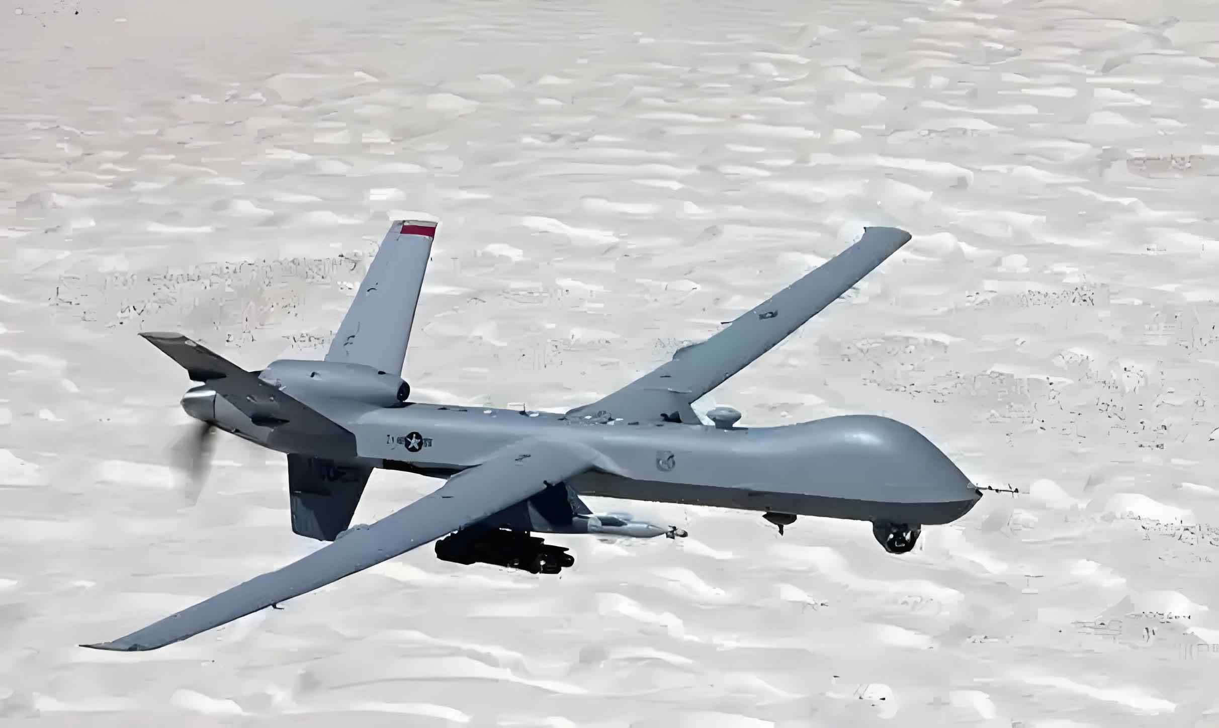
In modern defense systems, the military drone has become a pivotal asset, offering unmatched capabilities in surveillance, reconnaissance, and combat operations. However, the development of such advanced unmanned aerial vehicles poses significant financial challenges, primarily due to high technological complexity and limited historical data. Predicting the development cost of a military drone is crucial for budget planning, resource allocation, and strategic decision-making. Traditional cost estimation methods often struggle with the small sample sizes and multicollinearity among influencing factors, leading to inaccurate forecasts. In this article, I explore the application of Gram-Schmidt regression to address these issues, providing a robust framework for military drone cost prediction. This approach leverages orthogonal transformation to extract key parameters, mitigating the effects of multicollinearity and enhancing model reliability with scarce data. Through a detailed case study and comparisons with other techniques, I demonstrate the practicality and superiority of this method in forecasting military drone development expenses.
The growing reliance on military drone technology underscores the need for accurate cost prediction models. A military drone typically involves numerous design parameters, such as length, maximum takeoff weight, cruising speed, flight altitude, endurance, and payload, all of which interact in complex ways to influence development costs. With limited publicly available data—often due to confidentiality—conventional regression methods like ordinary least squares can fail due to multicollinearity, where predictor variables are highly correlated. This results in unstable coefficient estimates and poor generalization. Gram-Schmidt regression overcomes this by transforming correlated variables into an orthogonal set, selecting only the most informative features for the model. In the following sections, I will delve into the mathematical foundations of Gram-Schmidt regression, outline a step-by-step modeling process, and apply it to a real-world military drone dataset. The goal is to empower stakeholders with a tool that can deliver precise cost estimates even with minimal samples, thereby optimizing the development lifecycle of a military drone.
Gram-Schmidt regression is a multivariate statistical technique that combines Gram-Schmidt orthogonalization with linear regression to handle multicollinearity. Given a set of predictor variables \(x_1, x_2, \ldots, x_s\) and a response variable \(y\) (e.g., development cost of a military drone), the method iteratively constructs orthogonal vectors \(z_1, z_2, \ldots, z_m\) from the predictors, where \(m \leq s\). This orthogonalization process eliminates redundancy by ensuring that each new vector is uncorrelated with the previous ones. The regression is then performed on these orthogonal vectors, yielding stable coefficients that are later transformed back to the original predictor space. The core advantage lies in its ability to select only the most significant variables through hypothesis testing, reducing model complexity and improving interpretability. For military drone cost prediction, this means we can identify the key drivers of expense—such as flight altitude or length—while discarding less influential factors, even with a handful of samples. The mathematical formulation begins with the Gram-Schmidt transformation: for linearly independent variables \(x_1, x_2, \ldots, x_s\), we define:
$$z_1 = x_1,$$
$$z_2 = x_2 – \frac{x_2^T z_1}{z_1^T z_1} z_1,$$
$$z_3 = x_3 – \frac{x_3^T z_1}{z_1^T z_1} z_1 – \frac{x_3^T z_2}{z_2^T z_2} z_2,$$
$$\vdots$$
$$z_s = x_s – \sum_{k=1}^{s-1} \frac{x_s^T z_k}{z_k^T z_k} z_k.$$
This transformation can be expressed in matrix form as \(Z = X R^{-1}\), where \(Z = (z_1, z_2, \ldots, z_s)\), \(X = (x_1, x_2, \ldots, x_s)\), and \(R\) is an upper triangular matrix with elements \(r_{jk} = \frac{x_k^T z_j}{z_j^T z_j}\) for \(j < k\). In practice, to avoid numerical instability, a modified Gram-Schmidt process is often used, which updates vectors sequentially to preserve orthogonality. For military drone applications, this ensures that cost predictions remain accurate despite the high correlations among parameters like maximum takeoff weight and payload. The regression model on the orthogonal vectors is given by \(y = \beta_0 + \beta_1 z_1 + \cdots + \beta_m z_m\), which is then back-transformed to \(y = a_0 + a_1 x_1 + \cdots + a_m x_m\) for practical interpretation. By focusing on orthogonal components, Gram-Schmidt regression minimizes variance inflation and enhances prediction robustness—a critical need when estimating costs for a cutting-edge military drone.
To apply Gram-Schmidt regression to military drone development cost prediction, I follow a systematic modeling procedure. First, the predictor variables and cost data are centered to have zero mean, stabilizing the computation. Then, the algorithm iteratively selects variables based on their t-test significance in explaining cost variation. The steps are as follows:
- Centering: For each predictor \(x_j\) and the response \(y\), compute the centered versions by subtracting their means. This step standardizes the data and simplifies the orthogonalization.
- Initial Selection: For each centered predictor \(x_j\), treat it as \(z_{1j}\) and fit a simple linear regression with \(y\). Calculate the t-test statistic for each. The predictor with the largest absolute t-value that exceeds the critical threshold (e.g., \(t_{0.025}(n-2)\) for a 95% confidence level) is chosen as the first orthogonal vector \(z_1\). This variable has the strongest individual explanatory power for military drone cost.
- Iterative Orthogonalization and Selection: For the remaining predictors, perform Gram-Schmidt orthogonalization relative to the already selected vectors. For example, if \(z_1\) is chosen, compute \(z_{2j} = x_j – \frac{x_j^T z_1}{z_1^T z_1} z_1\) for each unselected \(x_j\). Then, fit a regression of \(y\) on \(z_1\) and each \(z_{2j}\), and evaluate the t-test for \(z_{2j}\). Select the one with the largest significant t-value as \(z_2\). Repeat this process, using the modified Gram-Schmidt update for numerical stability, until no remaining orthogonalized predictors pass the t-test.
- Model Fitting: Fit the final regression model using the selected orthogonal vectors: \(y = \beta_0 + \beta_1 z_1 + \cdots + \beta_m z_m\). The coefficients \(\beta_i\) are estimated via least squares, and the model’s goodness-of-fit (e.g., R-squared) is computed.
- Back-Transformation: Transform the model back to the original predictor space using the relation \(Z = X R^{-1}\). This yields a linear equation in terms of the original variables: \(y = a_0 + a_1 x_1 + \cdots + a_m x_m\), where \(a_i\) are derived from \(\beta_i\) and \(R\). This final model is used for predicting military drone development costs.
This procedure ensures that only the most informative parameters are included, reducing overfitting—a common issue with small datasets. For a military drone, typical predictors might include length, maximum takeoff weight, cruising speed, flight altitude, endurance, and payload. The iterative selection helps identify, say, flight altitude as a primary cost driver, while discarding redundant variables. To illustrate, consider a sample dataset of military drone characteristics and development costs, as shown in Table 1. The data are centered for analysis, and the Gram-Schmidt process is applied stepwise.
| Drone Model | Length (m) \(x_1\) | Max Takeoff Weight (kg) \(x_2\) | Cruising Speed (km/h) \(x_3\) | Flight Altitude (km) \(x_4\) | Endurance (h) \(x_5\) | Payload (kg) \(x_6\) | Development Cost ($B) \(y\) |
|---|---|---|---|---|---|---|---|
| A | 6.154 | 7625 | 206.6 | 9.414 | 19.71 | 504.5 | 1.436 |
| B | -2.096 | -3517 | -44.43 | -6.386 | -15.29 | -265.5 | -0.944 |
| C | -5.267 | -3837 | -132.4 | -6.386 | -18.29 | -230.5 | -1.324 |
| D | -3.076 | -3597 | -320.4 | -8.386 | -17.29 | -381.0 | -1.254 |
| E | 6.154 | 6398 | 297.6 | 10.01 | 23.71 | 509.5 | 1.916 |
| F | -2.746 | -96.7 | 204.6 | 4.814 | -10.29 | 54.5 | 0.376 |
| K (Test) | 0.874 | -2977 | -211.4 | -3.086 | 17.71 | -191.5 | -0.204 |
In this dataset, the correlation matrix (Table 2) reveals high multicollinearity among parameters, which can destabilize traditional regression. For instance, flight altitude and maximum takeoff weight have a correlation of 0.9447, emphasizing the need for orthogonalization in military drone cost modeling.
| Variable | \(x_1\) | \(x_2\) | \(x_3\) | \(x_4\) | \(x_5\) | \(x_6\) | \(y\) |
|---|---|---|---|---|---|---|---|
| \(x_1\) | 1.0000 | 0.9588 | 0.7256 | 0.8447 | 0.9819 | 0.9187 | 0.9145 |
| \(x_2\) | 0.9588 | 1.0000 | 0.8216 | 0.9447 | 0.9811 | 0.9841 | 0.9658 |
| \(x_3\) | 0.7256 | 0.8216 | 1.0000 | 0.9417 | 0.7881 | 0.8964 | 0.9131 |
| \(x_4\) | 0.8447 | 0.9447 | 0.9417 | 1.0000 | 0.9010 | 0.9743 | 0.9828 |
| \(x_5\) | 0.9819 | 0.9811 | 0.7881 | 0.9010 | 1.0000 | 0.9658 | 0.9522 |
| \(x_6\) | 0.9187 | 0.9841 | 0.8964 | 0.9743 | 0.9658 | 1.0000 | 0.9800 |
| \(y\) | 0.9145 | 0.9658 | 0.9131 | 0.9828 | 0.9522 | 0.9800 | 1.0000 |
Applying the Gram-Schmidt regression steps, I first center the data as in Table 1. Then, for each predictor, I compute the t-test statistics in simple linear regression with cost. The results (Table 3) show that flight altitude (\(x_4\)) has the highest absolute t-value (10.634), so it is selected as \(z_1\). This aligns with the intuition that altitude capability is a major cost factor for a military drone, as it involves advanced propulsion and materials.
| Predictor | \(x_1\) | \(x_2\) | \(x_3\) | \(x_4\) | \(x_5\) | \(x_6\) |
|---|---|---|---|---|---|---|
| t-Value | 4.520 | 7.447 | 4.479 | 10.634 | 6.234 | 9.862 |
Next, I orthogonalize the remaining predictors relative to \(z_1\) (centered \(x_4\)). For example, for length (\(x_1\)), compute \(z_{21} = x_1 – \frac{x_1^T z_1}{z_1^T z_1} z_1\). Then, fit regressions of \(y\) on \(z_1\) and each \(z_{2j}\), and obtain t-values (Table 4). The length (\(x_1\)) has the highest significant t-value (2.822), so it becomes \(z_2\). This step highlights that after accounting for altitude, length provides additional explanatory power for military drone cost, likely due to its impact on airframe size and complexity.
| Orthogonalized Predictor | \(z_{21}\) (from \(x_1\)) | \(z_{22}\) (from \(x_2\)) | \(z_{23}\) (from \(x_3\)) | \(z_{25}\) (from \(x_5\)) | \(z_{26}\) (from \(x_6\)) |
|---|---|---|---|---|---|
| t-Value | 2.822 | 1.355 | -0.352 | 2.594 | 1.114 |
Continuing, I orthogonalize further relative to \(z_1\) and \(z_2\), but none of the resulting vectors pass the t-test threshold (e.g., \(t_{0.025}(4) = 2.776\) for this stage). Thus, the selection stops with two variables: flight altitude and length. The regression model on the orthogonal vectors is:
$$y = 0.163941 z_1 + 0.083685 z_2.$$
Using the back-transformation \(Z = X R^{-1}\), where \(R\) is derived from the orthogonalization coefficients, I obtain the final cost prediction model in original terms:
$$y = 0.370923 + 0.083685 x_1 + 0.122466 x_4.$$
This model has an R-squared value of 0.990651, indicating excellent fit. The coefficients imply that, for a military drone, each additional meter of length increases development cost by approximately $0.0837 billion, and each kilometer of flight altitude adds about $0.1225 billion, holding other factors constant. These insights are valuable for designers aiming to balance performance and cost in a military drone project.
To validate the model, I apply it to the training data (Drones A-F) and compare predicted versus actual costs (Table 5). The errors range from 1.2% to 8.9%, with an average absolute error of 4.6%, demonstrating high accuracy. For instance, for Drone A, the predicted cost is $3.925 billion versus actual $3.71 billion, a 5.8% overestimate. Such precision is remarkable given the small sample size, underscoring the efficacy of Gram-Schmidt regression for military drone cost forecasting.
| Drone Model | Actual Cost ($B) | Predicted Cost ($B) | Error (%) |
|---|---|---|---|
| A | 3.71 | 3.925 | 5.8 |
| B | 1.33 | 1.300 | 2.2 |
| C | 0.95 | 1.035 | 8.9 |
| D | 1.02 | 0.973 | 4.6 |
| E | 4.19 | 3.999 | 4.6 |
| F | 2.65 | 2.617 | 1.2 |
For further testing, I use the holdout sample (Drone K), which represents a new military drone design. The model predicts a development cost of $1.9528 billion, compared to the actual value of $2.07 billion. This corresponds to a 5.57% error, which is competitive with other advanced methods. To contextualize, I compare Gram-Schmidt regression with several alternatives commonly used for military drone cost prediction: stepwise multiple regression (SMR), artificial neural networks (ANN) like BP and RBF, and partial least squares (PLS). The results are summarized in Table 6.
| Method | Predicted Cost for Drone K ($B) | Error (%) | Key Notes |
|---|---|---|---|
| Gram-Schmidt Regression | 1.9528 | 5.57 | Uses only 2 parameters; handles multicollinearity well. |
| Partial Least Squares (PLS) | 1.9616 | 5.24 | Uses all 6 parameters; similar accuracy but more complex. |
| Stepwise Multiple Regression (SMR) | 1.7181 | 17.0 | Higher error due to multicollinearity issues. |
| BP Neural Network | 1.89 | 8.7 | Requires more data; prone to overfitting. |
| RBF Neural Network | 1.96 | 5.3 | Accurate but computationally intensive. |
The comparison reveals that Gram-Schmidt regression achieves accuracy on par with PLS and RBF neural networks, while using only two predictors (length and flight altitude) instead of all six. This parsimony is a significant advantage for military drone applications, where data collection is often limited by secrecy or high costs. SMR performs poorly due to its vulnerability to multicollinearity, and ANN methods may overfit with small samples. Thus, Gram-Schmidt regression offers a balanced solution: it is simple, interpretable, and robust, making it ideal for early-stage cost estimation of a military drone when detailed information is scarce.
Beyond this case study, the Gram-Schmidt approach can be extended to incorporate additional factors relevant to military drone development, such as stealth features, communication systems, or autonomy levels. By orthogonalizing these variables, we can isolate their unique cost contributions. Moreover, the method can be adapted for nonlinear relationships by including interaction terms or polynomial transforms, though this may require more samples. For defense agencies, implementing such a model in a decision-support tool could streamline budgeting processes. For example, when prototyping a new military drone, engineers could input key parameters to obtain a reliable cost estimate, enabling trade-off analyses between performance and affordability. This proactive planning is essential in an era where military drone technology evolves rapidly, and cost overruns can jeopardize project viability.
In conclusion, Gram-Schmidt regression provides a powerful methodology for predicting the development cost of a military drone, especially under constraints of small sample sizes and high multicollinearity. By transforming correlated predictors into orthogonal components, it selects the most influential variables—such as flight altitude and length—and yields a stable, interpretable linear model. The case study demonstrates that this method can achieve prediction errors below 6% with only six training samples, outperforming stepwise regression and rivaling more complex techniques like neural networks. For stakeholders in defense and aerospace, adopting Gram-Schmidt regression can enhance cost forecasting accuracy, reduce financial risks, and support informed design choices. As military drone technology continues to advance, with trends toward swarming, AI integration, and longer endurance, robust cost prediction tools will become even more critical. Future research could explore hybrid models combining Gram-Schmidt regression with machine learning for even greater precision, or apply it to other cost phases like production or maintenance of a military drone. Ultimately, this approach underscores the value of statistical innovation in managing the economic challenges of modern defense systems.